Functional programming · Advanced (data.table)

Advanced · data.table

Author

Pablo Fuenzalida

Published

July 21, 2026

Functional programming · Advanced (data.table)

[i, j, by] when data get large.

Q1 · as.data.table() mindset

as.data.table() converts data frames without dropping columns; printing shows head and tail of large tables.

print(DTreef) # data.table print method

    transect_id   site     species count depth_m
         <char> <char>      <char> <int>   <num>
 1:         T01  North  Parrotfish     4     6.2
 2:         T01  North Surgeonfish    12     6.2
 3:         T01  North     Grouper     1     6.2
 4:         T01  North     Snapper     7     6.2
 5:         T01  North  Damselfish    21     6.2
 6:         T02  South  Parrotfish     6     5.2
 7:         T02  South Surgeonfish     7     5.2
 8:         T02  South     Grouper     2     5.2
 9:         T02  South     Snapper     9     5.2
10:         T02  South  Damselfish    20     5.2
11:         T03   East  Parrotfish     6     6.3
12:         T03   East Surgeonfish    13     6.3
13:         T03   East     Grouper     4     6.3
14:         T03   East     Snapper     5     6.3
15:         T03   East  Damselfish    26     6.3
16:         T04  North  Parrotfish     6     8.5
17:         T04  North Surgeonfish     8     8.5
18:         T04  North     Grouper     1     8.5
19:         T04  North     Snapper     2     8.5
20:         T04  North  Damselfish    17     8.5
21:         T05  South  Parrotfish    15    10.4
22:         T05  South Surgeonfish    10    10.4
23:         T05  South     Grouper     0    10.4
24:         T05  South     Snapper     4    10.4
25:         T05  South  Damselfish    22    10.4
26:         T06   East  Parrotfish    11     9.9
27:         T06   East Surgeonfish    10     9.9
28:         T06   East     Grouper     8     9.9
29:         T06   East     Snapper     8     9.9
30:         T06   East  Damselfish    26     9.9
31:         T07  North  Parrotfish     5     7.7
32:         T07  North Surgeonfish    13     7.7
33:         T07  North     Grouper     2     7.7
34:         T07  North     Snapper     4     7.7
35:         T07  North  Damselfish    25     7.7
36:         T08  South  Parrotfish     9     9.6
37:         T08  South Surgeonfish     8     9.6
38:         T08  South     Grouper     5     9.6
39:         T08  South     Snapper     5     9.6
40:         T08  South  Damselfish    22     9.6
41:         T09   East  Parrotfish     5     4.1
42:         T09   East Surgeonfish    14     4.1
43:         T09   East     Grouper     4     4.1
44:         T09   East     Snapper     1     4.1
45:         T09   East  Damselfish    26     4.1
46:         T10  North  Parrotfish     6     7.9
47:         T10  North Surgeonfish     8     7.9
48:         T10  North     Grouper     4     7.9
49:         T10  North     Snapper     5     7.9
50:         T10  North  Damselfish    25     7.9
51:         T11  South  Parrotfish     2    11.9
52:         T11  South Surgeonfish    15    11.9
53:         T11  South     Grouper     6    11.9
54:         T11  South     Snapper     5    11.9
55:         T11  South  Damselfish    24    11.9
56:         T12   East  Parrotfish    13     3.4
57:         T12   East Surgeonfish     9     3.4
58:         T12   East     Grouper     8     3.4
59:         T12   East     Snapper     4     3.4
60:         T12   East  Damselfish    18     3.4
    transect_id   site     species count depth_m

class(DTreef) # data.table and data.frame

[1] "data.table" "data.frame"

dim(DTreef) # rows and columns

[1] 60  5

Q2 · [i, j, by] core

The template DT[i, j, by] uses i to filter rows, j to compute, by to group.

DTreef[site == "North", .(mean_count = mean(count)), by = species]

       species mean_count
        <char>      <num>
1:  Parrotfish       5.25
2: Surgeonfish      10.25
3:     Grouper       2.00
4:     Snapper       4.50
5:  Damselfish      22.00

Also:

DTfish[port == "Cairns", .(mean_t = mean(tonnes)), by = species]

   species   mean_t
    <char>    <num>
1: Snapper 77.00000
2:   Shark 69.56667
3: Grouper 53.60000
4:    Tuna 13.90000

Also:

DTac[reef_zone == "Lagoon", .(total = sum(detections)), by = receiver]

   receiver total
     <char> <int>
1:       R9     3
2:       R1     3
3:      R11     6
4:       R2     3
5:      R12     7

Also:

DTbio[, .(max_depth = max(depth_m)), by = burst_id][1:5]

   burst_id max_depth
      <int>     <num>
1:        1  5.419779
2:        2  5.273251
3:        3  5.460373
4:        4  6.223412
5:        5  6.181104

Q3 · .N and .I

.N counts rows in the current group; .I holds indices for within-group positions.

DTac[, .N, by = animal_id] # rows per tag

   animal_id     N
      <char> <int>
1:      A101     8
2:      A102     8
3:      A103     8

DTac[, .(max_det = max(detections)), by = animal_id] # peak detection per tag

   animal_id max_det
      <char>   <int>
1:      A101       7
2:      A102       5
3:      A103       7

Q4 · .SD group columns

.SD is the Subset of Data for each group — all non-group columns inside j.

DTbio[, lapply(.SD, mean), by = burst_id, .SDcols = c("depth_m", "pitch_deg")]

    burst_id  depth_m  pitch_deg
       <int>    <num>      <num>
 1:        1 4.868771 -10.472410
 2:        2 4.429912  -4.306365
 3:        3 4.762483  -1.356978
 4:        4 5.566435  -1.278042
 5:        5 5.259435  -4.242083
 6:        6 4.977184   5.621892
 7:        7 5.124734  -3.856284
 8:        8 5.350061  -1.268552
 9:        9 5.604608   5.217801
10:       10 3.764709  -3.136650

Also:

DTreef[, lapply(.SD, mean), by = site, .SDcols = c("count", "depth_m")]

     site count depth_m
   <char> <num>   <num>
1:  North  8.80   7.575
2:  South  9.80   9.275
3:   East 10.95   5.925

Also:

DTfish[, .(min_t = min(tonnes), max_t = max(tonnes)), by = port]

         port min_t max_t
       <char> <num> <num>
1:     Cairns  13.9  97.3
2: Mooloolaba  23.0 144.5
3:     Broome  23.5  89.9

Q5 · := assign by reference

:= adds or updates columns in place without copying the whole table — fast but side-effectful.

DTfish[, kg := tonnes * 1000] # new column in place
head(DTfish[, .(species, tonnes, kg)]) # verify conversion

   species tonnes    kg
    <char>  <num> <num>
1: Snapper   75.7 75700
2: Grouper   79.6 79600
3:    Tuna   23.5 23500
4:   Shark   67.7 67700
5: Snapper   58.0 58000
6: Grouper   80.6 80600

Q6 · setorder() fast sort

setorder() sorts by reference; sorting biologging by burst and second prepares time-series ops.

setorder(DTbio, burst_id, seconds) # in-place sort
head(DTbio, 5) # inspect first rows

   burst_id seconds  depth_m  pitch_deg
      <int>   <int>    <num>      <num>
1:        1       0 4.798260 -27.611852
2:        1       1 5.065770 -20.483881
3:        1       2 4.755086 -17.718719
4:        1       3 4.730074  -6.960103
5:        1       4 4.665214 -24.308871

Q7 · Keys and binary search

A key indexes sorted column(s) — subsetting DT[id] uses binary search without merge syntax.

DTac_k <- copy(DTac) # avoid mutating shared object
setkey(DTac_k, animal_id) # sort and index
DTac_k["A101"] # fast row subset

Key: <animal_id>
   animal_id receiver detections reef_zone
      <char>   <char>      <int>    <char>
1:      A101      R11          5     Slope
2:      A101       R2          2     Crest
3:      A101       R6          7     Slope
4:      A101       R1          4     Crest
5:      A101       R5          5     Slope
6:      A101       R7          4     Slope
7:      A101       R7          4     Crest
8:      A101       R9          1     Crest

Q8 · merge() joins

merge() joins tables; with keys set, joins can be faster but always check nrow after.

ports <- data.table(port = c("Cairns", "Broome", "Mooloolaba"),
                      region = c("GBR", "NW", "SEQ"))
merge(DTfish, ports, by = "port", all.x = TRUE) # keep all landings

Key: <port>
          port  year species tonnes     kg region
        <char> <int>  <char>  <num>  <num> <char>
 1:     Broome  2018    Tuna   23.5  23500     NW
 2:     Broome  2019 Snapper   58.0  58000     NW
 3:     Broome  2020    Tuna   43.7  43700     NW
 4:     Broome  2020   Shark   89.9  89900     NW
 5:     Broome  2021 Grouper   74.5  74500     NW
 6:     Broome  2022 Snapper   49.8  49800     NW
 7:     Broome  2022   Shark   86.4  86400     NW
 8:     Broome  2023 Grouper   47.5  47500     NW
 9:     Broome  2023   Shark   45.1  45100     NW
10:     Cairns  2018 Snapper   75.7  75700    GBR
11:     Cairns  2018   Shark   67.7  67700    GBR
12:     Cairns  2019 Grouper   80.6  80600    GBR
13:     Cairns  2019   Shark   85.1  85100    GBR
14:     Cairns  2021 Snapper   97.3  97300    GBR
15:     Cairns  2021    Tuna   13.9  13900    GBR
16:     Cairns  2021   Shark   55.9  55900    GBR
17:     Cairns  2022 Grouper   26.6  26600    GBR
18:     Cairns  2023 Snapper   58.0  58000    GBR
19: Mooloolaba  2018 Grouper   79.6  79600    SEQ
20: Mooloolaba  2019    Tuna   53.4  53400    SEQ
21: Mooloolaba  2020 Snapper  144.5 144500    SEQ
22: Mooloolaba  2020 Grouper   23.0  23000    SEQ
23: Mooloolaba  2022    Tuna   39.7  39700    SEQ
24: Mooloolaba  2023    Tuna   29.2  29200    SEQ
          port  year species tonnes     kg region

Also:

meta <- data.table(animal_id = c("A101", "A102", "A103"), cohort = c(2023, 2023, 2024))
merge(DTac, meta, by = "animal_id", all.x = TRUE)[1:6]

Key: <animal_id>
   animal_id receiver detections reef_zone cohort
      <char>   <char>      <int>    <char>  <num>
1:      A101      R11          5     Slope   2023
2:      A101       R2          2     Crest   2023
3:      A101       R6          7     Slope   2023
4:      A101       R1          4     Crest   2023
5:      A101       R5          5     Slope   2023
6:      A101       R7          4     Slope   2023

Also:

site_meta <- data.table(site = c("North", "South", "East"), mgmt = c("MPA", "Open", "MPA"))
merge(DTreef, site_meta, by = "site")[1:6]

Key: <site>
     site transect_id     species count depth_m   mgmt
   <char>      <char>      <char> <int>   <num> <char>
1:   East         T03  Parrotfish     6     6.3    MPA
2:   East         T03 Surgeonfish    13     6.3    MPA
3:   East         T03     Grouper     4     6.3    MPA
4:   East         T03     Snapper     5     6.3    MPA
5:   East         T03  Damselfish    26     6.3    MPA
6:   East         T06  Parrotfish    11     9.9    MPA

Q9 · rbindlist() stack

rbindlist() binds a list of data.tables quickly — stack survey legs or batches.

north <- DTreef[site == "North"] # subset table
south <- DTreef[site == "South"] # another subset
rbindlist(list(north, south), use.names = TRUE) # combined table

    transect_id   site     species count depth_m
         <char> <char>      <char> <int>   <num>
 1:         T01  North  Parrotfish     4     6.2
 2:         T01  North Surgeonfish    12     6.2
 3:         T01  North     Grouper     1     6.2
 4:         T01  North     Snapper     7     6.2
 5:         T01  North  Damselfish    21     6.2
 6:         T04  North  Parrotfish     6     8.5
 7:         T04  North Surgeonfish     8     8.5
 8:         T04  North     Grouper     1     8.5
 9:         T04  North     Snapper     2     8.5
10:         T04  North  Damselfish    17     8.5
11:         T07  North  Parrotfish     5     7.7
12:         T07  North Surgeonfish    13     7.7
13:         T07  North     Grouper     2     7.7
14:         T07  North     Snapper     4     7.7
15:         T07  North  Damselfish    25     7.7
16:         T10  North  Parrotfish     6     7.9
17:         T10  North Surgeonfish     8     7.9
18:         T10  North     Grouper     4     7.9
19:         T10  North     Snapper     5     7.9
20:         T10  North  Damselfish    25     7.9
21:         T02  South  Parrotfish     6     5.2
22:         T02  South Surgeonfish     7     5.2
23:         T02  South     Grouper     2     5.2
24:         T02  South     Snapper     9     5.2
25:         T02  South  Damselfish    20     5.2
26:         T05  South  Parrotfish    15    10.4
27:         T05  South Surgeonfish    10    10.4
28:         T05  South     Grouper     0    10.4
29:         T05  South     Snapper     4    10.4
30:         T05  South  Damselfish    22    10.4
31:         T08  South  Parrotfish     9     9.6
32:         T08  South Surgeonfish     8     9.6
33:         T08  South     Grouper     5     9.6
34:         T08  South     Snapper     5     9.6
35:         T08  South  Damselfish    22     9.6
36:         T11  South  Parrotfish     2    11.9
37:         T11  South Surgeonfish    15    11.9
38:         T11  South     Grouper     6    11.9
39:         T11  South     Snapper     5    11.9
40:         T11  South  Damselfish    24    11.9
    transect_id   site     species count depth_m

Q10 · dcast() wide

dcast() pivots long to wide — detection totals by animal and receiver.

dcast(DTac, animal_id ~ receiver, value.var = "detections", fun.aggregate = sum, fill = 0)

Key: <animal_id>
   animal_id    R1   R11   R12    R2    R4    R5    R6    R7    R8    R9
      <char> <int> <int> <int> <int> <int> <int> <int> <int> <int> <int>
1:      A101     4     5     0     2     0     5     7     8     0     1
2:      A102     3     3     0     8     0     0     0     4     0     3
3:      A103     0     3    14     5     7     1     0     5     3     0

Q11 · melt() long

melt() unpivots wide tables — inverse of dcast for export pipelines.

wide <- dcast(DTfish[year == 2020], year ~ species, value.var = "tonnes", fill = 0)
melt(wide, id.vars = "year", variable.name = "species", value.name = "tonnes")

    year species tonnes
   <int>  <fctr>  <num>
1:  2020 Grouper   23.0
2:  2020   Shark   89.9
3:  2020 Snapper  144.5
4:  2020    Tuna   43.7

Q12 · shift() like lag

shift() moves values within groups — lag and lead for time series inside bursts.

DTbio[, depth_change := depth_m - shift(depth_m), by = burst_id]
DTbio[!is.na(depth_change), .(burst_id, seconds, depth_change)][1:8]

   burst_id seconds depth_change
      <int>   <int>        <num>
1:        1       1   0.26751027
2:        1       2  -0.31068411
3:        1       3  -0.02501225
4:        1       4  -0.06485909
5:        1       5   0.20001095
6:        1       6   0.17244104
7:        1       7   0.38211299
8:        1       8  -0.41157372

Also:

DTf <- copy(DTfish) # do not mutate capstone copy
DTf[, year := as.integer(year)] # ensure sort order
setorder(DTf, species, year)
DTf[, tonnes_lag := shift(tonnes), by = species]
DTf[!is.na(tonnes_lag), .(species, year, tonnes, tonnes_lag)][1:6]

   species  year tonnes tonnes_lag
    <char> <int>  <num>      <num>
1: Grouper  2019   80.6       79.6
2: Grouper  2020   23.0       80.6
3: Grouper  2021   74.5       23.0
4: Grouper  2022   26.6       74.5
5: Grouper  2023   47.5       26.6
6:   Shark  2019   85.1       67.7

Also:

DTac[, det_lag := shift(detections), by = animal_id]
DTac[!is.na(det_lag), .(animal_id, receiver, detections, det_lag)][1:6]

   animal_id receiver detections det_lag
      <char>   <char>      <int>   <int>
1:      A101       R2          2       5
2:      A101       R6          7       2
3:      A101       R1          4       7
4:      A101       R5          5       4
5:      A101       R7          4       5
6:      A101       R7          4       4

Q13 · fcase() like case_when

fcase() evaluates vectorised conditions top-down — fast alternative to dplyr case_when inside j.

DTfish[, size_bin := fcase(
  tonnes < 30, "small",
  tonnes < 70, "medium",
  default = "large"
)]
DTfish[, .N, by = size_bin] # bin counts

   size_bin     N
     <char> <int>
1:    large     9
2:    small     5
3:   medium    10

Also:

DTreef[, depth_bin := fcase(depth_m < 5, "shallow", depth_m < 12, "mid", default = "deep")]
DTreef[, .N, by = depth_bin]

   depth_bin     N
      <char> <int>
1:       mid    50
2:   shallow    10

Also:

DTac[, activity := fcase(detections == 0, "none", detections < 4, "low", default = "high")]
DTac[, .N, by = activity]

   activity     N
     <char> <int>
1:     high    12
2:      low    12

Q14 · Grouped chain ;

Curly braces with semicolons run multiple j expressions on the same filtered table — compact EDA.

east <- DTreef[site == "East"]
{
  east[, .(mean_depth = mean(depth_m), total_fish = sum(count))];
  east[, .(species, count)][order(-count)]
}

        species count
         <char> <int>
 1:  Damselfish    26
 2:  Damselfish    26
 3:  Damselfish    26
 4:  Damselfish    18
 5: Surgeonfish    14
 6: Surgeonfish    13
 7:  Parrotfish    13
 8:  Parrotfish    11
 9: Surgeonfish    10
10: Surgeonfish     9
11:     Grouper     8
12:     Snapper     8
13:     Grouper     8
14:  Parrotfish     6
15:     Snapper     5
16:  Parrotfish     5
17:     Grouper     4
18:     Grouper     4
19:     Snapper     4
20:     Snapper     1
        species count

Q15 · fread() big CSV

fread() reads large CSVs faster than read.csv from the same project-relative path.

reef_fread <- fread(data_path("reef_transects.csv")) # fast read; same path as
nrow(reef_fread) # should match DTreef

[1] 60

Q16 · Telemetry aggregation

Group acoustic detections by reef_zone and receiver — standard passive telemetry summaries.

tel <- DTac[, .(total = sum(detections), n = .N), by = .(reef_zone, receiver)]
tel[order(-total)][1:10] # top ten cells

    reef_zone receiver total     n
       <char>   <char> <int> <int>
 1:     Slope       R7    11     3
 2:     Crest       R2     7     2
 3:     Slope       R6     7     1
 4:     Crest      R12     7     1
 5:    Lagoon      R12     7     1
 6:     Slope       R4     7     1
 7:     Crest       R7     6     2
 8:    Lagoon      R11     6     3
 9:     Slope      R11     5     1
10:     Slope       R5     5     1

Q17 · Fishery by year

Annual summaries with by = year mirror agency reports — sum tonnes and count records separately.

DTfish[, .(tonnes = sum(tonnes), records = .N), by = year][order(year)]

    year tonnes records
   <int>  <num>   <int>
1:  2018  246.5       4
2:  2019  277.1       4
3:  2020  301.1       4
4:  2021  241.6       4
5:  2022  202.5       4
6:  2023  179.8       4

Q18 · Biologging rolling mean

Rolling means smooth depth noise along bursts — three-point centred window using shift sums.

DTbio[, roll_depth := (shift(depth_m, 1, type = "lag") + depth_m + shift(depth_m, 1, type = "lead")) / 3, by = burst_id]
DTbio[!is.na(roll_depth), .(burst_id, seconds, depth_m, roll_depth)][1:8]

   burst_id seconds  depth_m roll_depth
      <int>   <int>    <num>      <num>
1:        1       1 5.065770   4.873038
2:        1       2 4.755086   4.850310
3:        1       3 4.730074   4.716791
4:        1       4 4.665214   4.753504
5:        1       5 4.865225   4.856035
6:        1       6 5.037666   5.107557
7:        1       7 5.419779   5.155217
8:        1       8 5.008206   5.164646

Q19 · .BY in j

.BY exposes current by-group values inside j — handy for labels without repeating columns.

DTac[, .(
  zone = .BY[[1]],
  total = sum(detections)
), by = reef_zone]

   reef_zone   zone total
      <char> <char> <int>
1:     Slope  Slope    43
2:     Crest  Crest    26
3:    Lagoon Lagoon    22

Q20 · data.table capstone

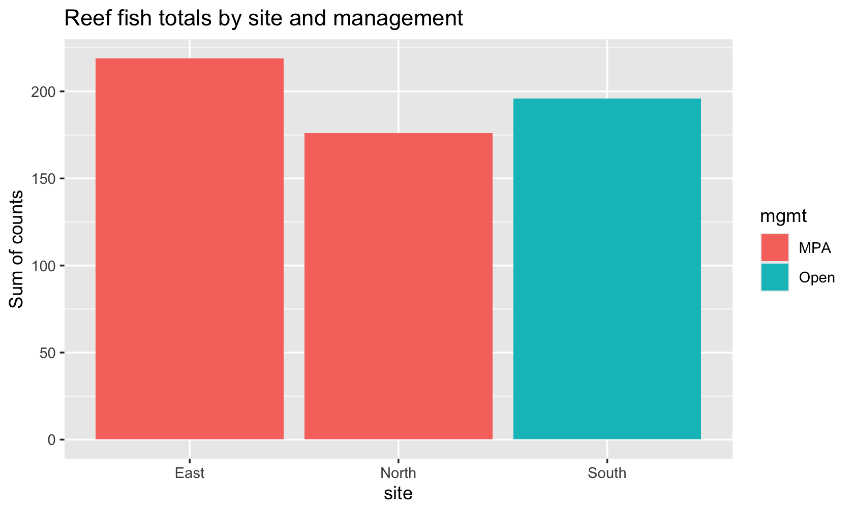
Capstone combines aggregation, merge, and ggplot on reef totals — meeting-ready output you verify before AI optimises.

meta <- data.table(site = c("North", "South", "East"), mgmt = c("MPA", "Open", "MPA"))
reef_sum <- DTreef[, .(total = sum(count), species_n = uniqueN(species)), by = site]
out <- merge(reef_sum, meta, by = "site")
ggplot(as.data.frame(out), aes(x = site, y = total, fill = mgmt)) +
  geom_col() +
  labs(title = "Reef fish totals by site and management", y = "Sum of counts")