Functional programming · Intermediate (dplyr)

Intermediate track — twenty quests on mutate, group_by, lead/lag, joins, and pivots.

Functional programming · Intermediate (dplyr)

dplyr verbs read like sentences: select columns, filter rows, mutate new variables, summarise within groups. This level builds verb-by-verb mental models so you can read, write, and fix pipelines on reef, fishery, acoustic, and biologging data.

Learning progresses when you connect new syntax to problems you already solved in base R (Bransford et al., 2000). Each quest (~10 minutes) ends with a prediction you can check: row counts, column names, or a plot you recognise from the field.

Treat dplyr as a contract with your data: every verb documents an intent. Choosing which steps belong in a pipeline is the same scientific reasoning habit Klahr and Dunbar describe in experiment design — applied to code.

Harder verbs (group_by, lead/lag, case_when, across, joins, pivots) include multiple worked examples on different ecological tables.

Q1 · select() & rename()

The select() verb keeps or drops columns by name, type, or tidy helpers like starts_with(). rename() changes names without touching other columns — cleaner than reassigning names(df) when AI adds a typo.

Before typing select(), list which columns your analysis actually needs. Extra columns increase cognitive load when reading joins downstream.

We trim the reef table to identifiers and abundance, renaming count to n_fish for publication-ready headers.

reef_sl <- reef |>                                 # start with reef transect data
  select(transect_id, site, species, count, depth_m) |>  # keep core columns only
  rename(n_fish = count)                               # clearer name for counts
glimpse(reef_sl)                                       # confirm column names

Rows: 60
Columns: 5
$ transect_id <chr> "T01", "T01", "T01", "T01", "T01", "T02", "T02", "T02", "T…
$ site        <chr> "North", "North", "North", "North", "North", "South", "Sou…
$ species     <chr> "Parrotfish", "Surgeonfish", "Grouper", "Snapper", "Damsel…
$ n_fish      <int> 4, 12, 1, 7, 21, 6, 7, 2, 9, 20, 6, 13, 4, 5, 26, 6, 8, 1,…
$ depth_m     <dbl> 6.2, 6.2, 6.2, 6.2, 6.2, 5.2, 5.2, 5.2, 5.2, 5.2, 6.3, 6.3…

Q2 · filter() rows

filter() keeps rows where a logical condition is TRUE. Unlike base subsetting, dplyr verbs error helpfully when you use = instead of == in many contexts — but AI still generates wrong variable names.

Always check nrow() before and after a filter; it is cheap feedback on whether your logic matches the field protocol.

Keep East site transects with depth at least five metres.

reef_east_deep <- reef |>                        # pipe data into filter
  filter(site == "East", depth_m >= 5)                  # both conditions must hold
nrow(reef_east_deep)                                    # rows retained

[1] 10

distinct(reef_east_deep, transect_id)                   # which transects survived

  transect_id
1         T03
2         T06

Q3 · mutate() new columns

mutate() adds or replaces columns while keeping all rows — the workhorse for unit conversions, binary flags, and intermediate biology.

Mutate is vectorised: each expression sees whole columns. That matches how R thinks and differs from row-wise loops unless you call rowwise().

Add kg from tonnes on fishery landings and a heavy-landing flag.

fishery_mut <- fishery |>                        # fisheries landing table
  mutate(
    kg = tonnes * 1000,                                 # metric conversion
    heavy = tonnes > 80                                 # logical flag for large trips
  )
summary(fishery_mut$kg)                                 # QC numeric range

   Min. 1st Qu.  Median    Mean 3rd Qu.    Max. 
  13900   42700   56950   60358   79850  144500 

Q4 · transmute() keep only new

transmute() is mutate that drops all previous columns — useful when you only want derived variables for modelling or export.

AI sometimes chains select() after mutate() when transmute() would be clearer; recognising the verb saves clutter.

Extract animal id and scaled detections from acoustic data.

acoustic_derived <- acoustic |>                  # acoustic telemetry rows
  transmute(
    animal_id,                                          # keep tag id
    detections_scaled = detections / max(detections)  # scale to 0-1 for plotting
  )
head(acoustic_derived)                                  # only new columns remain

  animal_id detections_scaled
1      A101         0.7142857
2      A101         0.2857143
3      A101         1.0000000
4      A101         0.5714286
5      A101         0.7142857
6      A101         0.5714286

Q5 · arrange() sort rows

arrange() sorts rows using order() logic under the hood — including desc() for decreasing sort.

Sorting is not cosmetic: time-series plots and lead()/lag() in later quests assume intentional row order within groups.

Order biologging seconds within each burst.

biolog_ord <- biolog |>                          # biologging burst series
  arrange(burst_id, seconds)                            # time order inside bursts
head(biolog_ord, 6)                                     # verify first burst sequence

  burst_id seconds  depth_m  pitch_deg
1        1       0 4.798260 -27.611852
2        1       1 5.065770 -20.483881
3        1       2 4.755086 -17.718719
4        1       3 4.730074  -6.960103
5        1       4 4.665214 -24.308871
6        1       5 4.865225   3.147493

Q6 · distinct() unique rows

distinct() returns unique rows, optionally by a subset of columns — dplyr’s answer to unique() on data frames.

Use it after joins to confirm you did not duplicate keys — a common AI join mistake.

List unique site–depth combinations on reef surveys.

sites_depths <- reef |>                          # reef data
  distinct(site, depth_m) |>                            # one row per combo
  arrange(site, depth_m)                                # readable table
sites_depths                                            # print result

    site depth_m
1   East     3.4
2   East     4.1
3   East     6.3
4   East     9.9
5  North     6.2
6  North     7.7
7  North     7.9
8  North     8.5
9  South     5.2
10 South     9.6
11 South    10.4
12 South    11.9

Q7 · slice() row index

slice() picks rows by position; helpers like slice_max() pick top values per group when combined with group_by().

Index slicing is fragile if row order changes — document why order is stable before slicing.

Take the deepest reading per burst from biologging.

deepest <- biolog |>                             # all burst seconds
  group_by(burst_id) |>                                 # partition by burst
  slice_max(depth_m, n = 1, with_ties = FALSE)          # deepest single row each
deepest                                                 # one row per burst_id

# A tibble: 10 × 4
# Groups:   burst_id [10]
   burst_id seconds depth_m pitch_deg
      <int>   <int>   <dbl>     <dbl>
 1        1       7    5.42   -11.1  
 2        2      16    5.27     2.45 
 3        3      17    5.46     5.95 
 4        4       9    6.22   -16.9  
 5        5      17    6.18     3.08 
 6        6       0    6.30    12.3  
 7        7       2    5.71    -7.25 
 8        8      14    6.46    10.1  
 9        9      15    6.43     0.482
10       10       0    6.43    23.5  

Q8 · group_by() + summarise()

group_by() marks grouping columns; summarise() collapses each group to one row. Forgetting to ungroup is a classic AI bug that poisons later mutates.

After summarise, ask: ‘How many rows should I have?’ — compare to n_distinct(group_cols).

Mean fish count per site on reef data.

reef_site_mean <- reef |>                        # transect counts
  group_by(site) |>                                     # groups: North, South, East
  summarise(
    mean_count = mean(count),                           # average abundance
    n_rows = n(),                                       # rows contributing
    .groups = "drop"                                    # avoid sticky grouping
  )
reef_site_mean                                          # three rows expected

# A tibble: 3 × 3
  site  mean_count n_rows
  <chr>      <dbl>  <int>
1 East        11.0     20
2 North        8.8     20
3 South        9.8     20

Example 2 — fishery: mean tonnes landed per species.

fishery |>
  group_by(species) |>
  summarise(mean_t = mean(tonnes), n = n(), .groups = "drop")

# A tibble: 4 × 3
  species mean_t     n
  <chr>    <dbl> <int>
1 Grouper   55.3     6
2 Shark     71.7     6
3 Snapper   80.6     6
4 Tuna      33.9     6

Example 3 — acoustic: total detections per animal_id (sum, not mean — common telemetry summary).

acoustic |>
  group_by(animal_id) |>
  summarise(total_det = sum(detections), n_receivers = n_distinct(receiver), .groups = "drop")

# A tibble: 3 × 3
  animal_id total_det n_receivers
  <chr>         <int>       <int>
1 A101             32           7
2 A102             21           5
3 A103             38           7

Q9 · count() quick tables

count() is shorthand for group_by() + summarise(n = n()), ideal for frequency tables before modelling.

Run counts before chi-square tests or occupancy models to spot empty cells early.

Count acoustic detections rows by reef zone and receiver.

det_counts <- acoustic |>                        # telemetry table
  count(reef_zone, receiver, name = "rows", sort = TRUE)  # sorted frequencies
head(det_counts, 10)                                    # busiest combinations

   reef_zone receiver rows
1     Lagoon      R11    3
2      Slope       R7    3
3      Crest       R2    2
4      Crest       R7    2
5      Crest       R1    1
6      Crest      R12    1
7      Crest       R5    1
8      Crest       R9    1
9     Lagoon       R1    1
10    Lagoon      R12    1

Q10 · lead() & lag() time series

lag() shifts values backward in row order; lead() shifts forward — essential for step changes in depth or pitch along seconds.

They require sorted data within groups — you arranged biologging in Q5 for this reason.

Compute second-to-second depth change within bursts.

depth_steps <- biolog_ord |>                     # sorted biolog data
  group_by(burst_id) |>                                 # independent time within burst
  mutate(depth_change = depth_m - lag(depth_m)) |>    # current minus previous
  filter(!is.na(depth_change))                          # drop first second each burst
head(depth_steps, 8)                                    # inspect changes

# A tibble: 8 × 5
# Groups:   burst_id [1]
  burst_id seconds depth_m pitch_deg depth_change
     <int>   <int>   <dbl>     <dbl>        <dbl>
1        1       1    5.07   -20.5         0.268 
2        1       2    4.76   -17.7        -0.311 
3        1       3    4.73    -6.96       -0.0250
4        1       4    4.67   -24.3        -0.0649
5        1       5    4.87     3.15        0.200 
6        1       6    5.04    -4.98        0.172 
7        1       7    5.42   -11.1         0.382 
8        1       8    5.01     0.713      -0.412 

Example 2 — biologging pitch: same pattern on pitch_deg within bursts.

biolog_ord |>
  group_by(burst_id) |>
  mutate(pitch_step = pitch_deg - lag(pitch_deg)) |>
  filter(!is.na(pitch_step)) |>
  slice_head(n = 4)

# A tibble: 40 × 5
# Groups:   burst_id [10]
   burst_id seconds depth_m pitch_deg pitch_step
      <int>   <int>   <dbl>     <dbl>      <dbl>
 1        1       1    5.07    -20.5       7.13 
 2        1       2    4.76    -17.7       2.77 
 3        1       3    4.73     -6.96     10.8  
 4        1       4    4.67    -24.3     -17.3  
 5        2       1    4.09    -18.1     -32.1  
 6        2       2    4.46     -7.60     10.5  
 7        2       3    4.28      5.71     13.3  
 8        2       4    4.05      5.21     -0.507
 9        3       1    4.49    -25.3     -23.7  
10        3       2    4.99      2.51     27.8  
# ℹ 30 more rows

Example 3 — fishery (file order): lag(tonnes) within species to compare consecutive landing records in the CSV order (not true calendar time — always check sort first).

fishery |>
  arrange(species, year) |>
  group_by(species) |>
  mutate(tonnes_prev = lag(tonnes), delta_t = tonnes - lag(tonnes)) |>
  filter(!is.na(delta_t)) |>
  head(6)

# A tibble: 6 × 6
# Groups:   species [2]
   year species tonnes port       tonnes_prev delta_t
  <int> <chr>    <dbl> <chr>            <dbl>   <dbl>
1  2019 Grouper   80.6 Cairns            79.6     1  
2  2020 Grouper   23   Mooloolaba        80.6   -57.6
3  2021 Grouper   74.5 Broome            23      51.5
4  2022 Grouper   26.6 Cairns            74.5   -47.9
5  2023 Grouper   47.5 Broome            26.6    20.9
6  2019 Shark     85.1 Cairns            67.7    17.4

Q11 · if_else() & case_when()

if_else() is strict typed ifelse for two branches; case_when() handles multiple rules readable top-to-bottom — like nested QC without spaghetti.

Order matters in case_when(): first match wins, mirroring priority QC protocols.

Classify fishery landings into size bins for reporting.

fishery_bins <- fishery |>                       # landing records
  mutate(
    size_bin = case_when(
      tonnes < 30 ~ "small",                            # first matching rule
      tonnes < 70 ~ "medium",
      TRUE ~ "large"                                    # catch-all required
    )
  )
count(fishery_bins, size_bin)                           # bin frequencies

  size_bin  n
1    large  9
2   medium 10
3    small  5

Example 2 — reef depth zones with case_when() (MPA planning bins).

reef |>
  mutate(depth_zone = case_when(
    depth_m < 5 ~ "upper",
    depth_m < 10 ~ "mid",
    TRUE ~ "deep"
  )) |>
  count(site, depth_zone)

   site depth_zone  n
1  East        mid 10
2  East      upper 10
3 North        mid 20
4 South       deep 10
5 South        mid 10

Example 3 — acoustic activity with strict if_else() (two outcomes only).

acoustic |>
  mutate(active = if_else(detections >= 4, "high", "low")) |>
  count(reef_zone, active)

  reef_zone active n
1     Crest   high 4
2     Crest    low 4
3    Lagoon   high 1
4    Lagoon    low 6
5     Slope   high 7
6     Slope    low 2

Q12 · across() many columns

across() applies a function to multiple columns selected by name or helper — the tidy way to scale numeric columns without copy-paste.

Watch types: across(where(is.numeric)) avoids accidentally rounding character columns AI mislabeled.

Z-score numeric columns in biologging (within full table demo).

biolog_scaled <- biolog |>                       # burst time series
  mutate(across(c(depth_m, pitch_deg), ~ as.numeric(scale(.))))  # z-scores
summary(biolog_scaled$depth_m)                          # mean ~0, sd ~1

    Min.  1st Qu.   Median     Mean  3rd Qu.     Max. 
-3.65895 -0.46600  0.08311  0.00000  0.65907  1.77198 

Example 2 — reef: scale count and depth_m after filtering site == "North".

reef |>
  filter(site == "North") |>
  mutate(across(c(count, depth_m), ~ as.numeric(scale(.)))) |>
  summarise(across(c(count, depth_m), mean))

          count       depth_m
1 -8.881784e-17 -1.021405e-15

Example 3 — fishery: across with mean and sd on tonnes by port.

fishery |>
  group_by(port) |>
  summarise(across(tonnes, list(mean = mean, sd = sd), .names = "{.fn}_{.col}"))

# A tibble: 3 × 3
  port       mean_tonnes sd_tonnes
  <chr>            <dbl>     <dbl>
1 Broome            57.6      21.9
2 Cairns            62.3      27.3
3 Mooloolaba        61.6      45.3

Q13 · group_modify() custom tables

group_modify() passes each group as a tibble to a function that returns a tibble — when summarise() is too limited for custom row-wise tables.

Use sparingly; it is slower than vectorised summaries but mirrors base lapply on splits explicitly.

Per species on reef: min, max, and range of counts.

sp_range <- reef |>                             # species counts
  group_by(species) |>                                  # one group per species
  group_modify(~ {                                      # .x is species subset
    tibble(                                             # return tibble shape
      min_n = min(.x$count),
      max_n = max(.x$count),
      range_n = max(.x$count) - min(.x$count)
    )
  })
sp_range                                                # custom table per species

# A tibble: 5 × 4
# Groups:   species [5]
  species     min_n max_n range_n
  <chr>       <int> <int>   <int>
1 Damselfish     17    26       9
2 Grouper         0     8       8
3 Parrotfish      2    15      13
4 Snapper         1     9       8
5 Surgeonfish     7    15       8

Example 2 — fishery: range of tonnes per port.

fishery |>
  group_by(port) |>
  group_modify(~ tibble(min_t = min(.x$tonnes), max_t = max(.x$tonnes)))

# A tibble: 3 × 3
# Groups:   port [3]
  port       min_t max_t
  <chr>      <dbl> <dbl>
1 Broome      23.5  89.9
2 Cairns      13.9  97.3
3 Mooloolaba  23   144. 

Example 3 — acoustic: top receiver by summed detections per animal_id.

acoustic |>
  group_by(animal_id) |>
  group_modify(~ {
    .x |>
      group_by(receiver) |>
      summarise(d = sum(detections), .groups = "drop") |>
      slice_max(d, n = 1)
  })

# A tibble: 3 × 3
# Groups:   animal_id [3]
  animal_id receiver     d
  <chr>     <chr>    <int>
1 A101      R7           8
2 A102      R2           8
3 A103      R12         14

Q14 · mutate(.by = )

Dplyr 1.1+ mutate(.by = ) groups temporarily for one mutate without sticky group_by() — great for within-animal or within-burst calculations.

It reduces AI-generated group_by() + ungroup() boilerplate when only one verb needs groups.

Centre detections within each animal id.

acoustic_cent <- acoustic |>                     # detection rows
  mutate(
    det_cent = detections - mean(detections),           # overall mean if no .by
    det_by_an = detections - mean(detections), .by = animal_id  # within-tag mean
  )
head(acoustic_cent)                                     # compare columns

  animal_id receiver detections reef_zone det_cent det_by_an
1      A101      R11          5     Slope        1         1
2      A101       R2          2     Crest       -2        -2
3      A101       R6          7     Slope        3         3
4      A101       R1          4     Crest        0         0
5      A101       R5          5     Slope        1         1
6      A101       R7          4     Slope        0         0

Q15 · left_join() metadata

left_join() keeps all rows from the left table and adds matching columns from the right — the join ecologists use for tagging metadata.

Always join on explicit keys; verify row count unchanged unless you expect duplication.

Attach a synthetic port region lookup to fishery landings.

ports <- tibble(                                 # small lookup table
  port = c("Cairns", "Broome", "Mooloolaba"),
  region = c("GBR", "NW", "SEQ")
)
fishery_geo <- fishery |>                               # landings left side
  left_join(ports, by = "port")                         # add region column
count(fishery_geo, region)                              # rows per region

  region n
1    GBR 9
2     NW 9
3    SEQ 6

Example 2 — acoustic: join tag metadata (hypothetical deployment reef) onto detections.

tag_meta <- tibble(
  animal_id = c("A101", "A102", "A103"),
  tag_type = c("V16", "V16", "V13")
)
acoustic |>
  left_join(tag_meta, by = "animal_id") |>
  count(tag_type, reef_zone)

  tag_type reef_zone n
1      V13     Crest 2
2      V13    Lagoon 2
3      V13     Slope 4
4      V16     Crest 6
5      V16    Lagoon 5
6      V16     Slope 5

Example 3 — reef: join site management zone onto transects.

site_meta <- tibble(site = c("North", "South", "East"), zone = c("MPA", "Open", "MPA"))
reef |>
  left_join(site_meta, by = "site") |>
  distinct(site, zone)

   site zone
1 North  MPA
2 South Open
3  East  MPA

Q16 · bind_rows() stack surveys

bind_rows() stacks compatible data frames — binding years or survey legs after harmonising column names.

Unlike rbind(), it handles missing columns by filling NA — know which behaviour you want before AI stacks mismatched CSVs.

Stack reef subset with itself renamed as pseudo replicate survey.

reef_a <- reef |> filter(site == "North")       # first leg
reef_b <- reef |> filter(site == "South") |>             # second leg
  mutate(transect_id = paste0(transect_id, "_b"))       # avoid id collision
stacked <- bind_rows(
  mutate(reef_a, leg = "north"),
  mutate(reef_b, leg = "south")
)                                                     # tagged stack
nrow(stacked)                                           # combined rows

[1] 40

Q17 · pivot_longer()

pivot_longer() melts wide columns into key-value rows — standard before ggplot when measurements live in many columns.

Name the names_to and values_to columns deliberately so AI-generated plots have sensible axis labels.

Wide fishery: columns per species for one year slice (constructed) then pivot.

wide_demo <- fishery |>                          # long landings
  filter(year == 2020) |>                               # single year
  select(species, tonnes) |>                              # minimal columns
  pivot_wider(names_from = species, values_from = tonnes)  # wide for exercise
long_demo <- wide_demo |>                               # now melt back
  pivot_longer(everything(), names_to = "species", values_to = "tonnes", values_drop_na = TRUE)
long_demo                                               # long form restored

# A tibble: 4 × 2
  species tonnes
  <chr>    <dbl>
1 Snapper  144. 
2 Grouper   23  
3 Tuna      43.7
4 Shark     89.9

Example 2 — reef: one transect wide by species, then long again for plotting.

reef |>
  filter(transect_id == "T01") |>
  select(species, count) |>
  pivot_wider(names_from = species, values_from = count) |>
  pivot_longer(everything(), names_to = "species", values_to = "count")

# A tibble: 5 × 2
  species     count
  <chr>       <int>
1 Parrotfish      4
2 Surgeonfish    12
3 Grouper         1
4 Snapper         7
5 Damselfish     21

Example 3 — biologging: pivot_longer() on depth_m and pitch_deg for one burst (sensor comparison).

biolog |>
  filter(burst_id == 1) |>
  select(seconds, depth_m, pitch_deg) |>
  pivot_longer(c(depth_m, pitch_deg), names_to = "sensor", values_to = "value") |>
  head(6)

# A tibble: 6 × 3
  seconds sensor     value
    <int> <chr>      <dbl>
1       0 depth_m     4.80
2       0 pitch_deg -27.6 
3       1 depth_m     5.07
4       1 pitch_deg -20.5 
5       2 depth_m     4.76
6       2 pitch_deg -17.7 

Q18 · pivot_wider()

pivot_wider() spreads key-value pairs into columns — useful for occupancy matrices or wide export to Excel.

Watch for duplicate keys; pivot will error or aggregate depending on settings — check values_fn.

Acoustic: detections per animal-receiver pair as wide matrix.

ac_wide <- acoustic |>                          # long detections
  group_by(animal_id, receiver) |>                      # unique pairs
  summarise(dets = sum(detections), .groups = "drop") |> # aggregate duplicates
  pivot_wider(names_from = receiver, values_from = dets, values_fill = 0)
ac_wide                                                 # wide receiver columns

# A tibble: 3 × 11
  animal_id    R1   R11    R2    R5    R6    R7    R9   R12    R4    R8
  <chr>     <int> <int> <int> <int> <int> <int> <int> <int> <int> <int>
1 A101          4     5     2     5     7     8     1     0     0     0
2 A102          3     3     8     0     0     4     3     0     0     0
3 A103          0     3     5     1     0     5     0    14     7     3

Q19 · replace_na() & coalesce()

replace_na() swaps NA for a value; coalesce() picks the first non-NA from several columns — handy when merging sensor streams.

Document why NA existed: missing vs not applicable changes whether replace is scientific.

Replace NA in optional column after join simulation on reef depths.

reef_na <- reef |>                              # original reef
  mutate(depth_m = if_else(species == "Grouper", NA_real_, depth_m))  # inject NA demo
reef_fix <- reef_na |>                                  # repair for plotting
  mutate(depth_m = replace_na(depth_m, median(reef$depth_m, na.rm = TRUE)))
sum(is.na(reef_fix$depth_m))                            # should be zero

[1] 0

Q20 · dplyr capstone pipeline

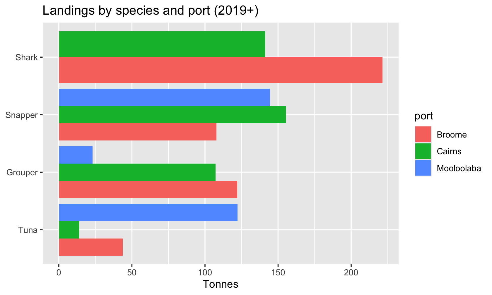
Capstone: one readable pipeline from raw landings to a figure — the shape of a methods supplement AI should not invent without your sign-off.

Read bottom-up: what object enters ggplot(), what one row represents, which filters happened.

Fishery totals by species and port with plot.

cap <- fishery |>                               # start landings
  filter(year >= 2019) |>                               # recent years
  group_by(species, port) |>                            # reporting cells
  summarise(total_t = sum(tonnes), .groups = "drop") |> # summed tonnes
  arrange(desc(total_t))                                # largest first
ggplot(cap, aes(x = reorder(species, total_t), y = total_t, fill = port)) +
  geom_col(position = "dodge") +                        # compare ports
  coord_flip() +                                        # readable labels
  labs(title = "Landings by species and port (2019+)", x = NULL, y = "Tonnes")