Functional programming · Beginner (Base R)

Beginner · base R

Author

Pablo Fuenzalida

Published

July 21, 2026

Functional programming · Beginner (Base R)

Base R: vectors, [, apply, loops. ~10 min/quest; harder quests show 2–3 datasets.

Q1 · Vectors, names, and types

counts <- reef$count
sites <- reef$site # site names
names(counts) <- NULL
length(counts)

[1] 60

typeof(counts) # internal storage type

[1] "integer"

unique(sites)

[1] "North" "South" "East"

Q2 · Subsetting `[`, `$`, `[[`

recent <- fishery[fishery$year >= 2020, ]
tons_snapper <- fishery$tonnes[fishery$species == "Snapper"] # vector of Snapper landings
cols <- fishery[, c("year", "species", "tonnes")]
first_port <- fishery[["port"]][1]
nrow(recent)

[1] 16

Q3 · if, else, and ifelse

high <- acoustic$detections > 4
flag <- ifelse(high, "revisit", "ok")
table(flag)

flag
     ok revisit 
     15       9

if (any(is.na(acoustic$detections))) {
  message("Found missing detection counts")
} else {
  message("No NA in detections")
}

Ex 2.

reef$depth_class <- ifelse(reef$depth_m < 6, "shallow", "deep")
table(reef$depth_class)


   deep shallow 
     45      15

Ex 2.

fishery$big_trip <- ifelse(fishery$tonnes >= 50, "major", "routine")
if (any(fishery$tonnes > 100, na.rm = TRUE)) {
  message("At least one landing exceeds 100 t — check port log")
}
table(fishery$big_trip)


  major routine 
     14      10

Q4 · for loops on real rows

burst_ids <- unique(biolog$burst_id)
mean_depths <- numeric(length(burst_ids))
for (i in seq_along(burst_ids)) {
  bid <- burst_ids[i]
  rows <- biolog$depth_m[biolog$burst_id == bid]
  mean_depths[i] <- mean(rows)
}
names(mean_depths) <- paste0("burst_", burst_ids)
mean_depths

 burst_1  burst_2  burst_3  burst_4  burst_5  burst_6  burst_7  burst_8 
4.868771 4.429912 4.762483 5.566435 5.259435 4.977184 5.124734 5.350061 
 burst_9 burst_10 
5.604608 3.764709

Ex 2.

ports <- unique(fishery$port) # each landing port once
port_tot <- numeric(length(ports)) # pre-allocate totals
for (j in seq_along(ports)) {
  p <- ports[j]
  port_tot[j] <- sum(fishery$tonnes[fishery$port == p])
}
names(port_tot) <- ports
port_tot

    Cairns Mooloolaba     Broome 
     560.8      369.4      518.4

Ex 2.

tags <- unique(acoustic$animal_id) # tagged animals in file
tag_sum <- numeric(length(tags)) # one total per tag
for (k in seq_along(tags)) {
  tag_sum[k] <- sum(acoustic$detections[acoustic$animal_id == tags[k]])
}
names(tag_sum) <- tags
tag_sum

A101 A102 A103 
  32   21   38

Q5 · Writing functions

tonnes_to_kg <- function(tonnes, factor = 1000) { # factor default matches metric
  tonnes * factor
}
fishery$kg <- tonnes_to_kg(fishery$tonnes) # apply to landing weights
sum(fishery$kg, na.rm = TRUE) # total kg landed in file

[1] 1448600

tonnes_to_kg(1.5) # scalar check: expect 1500

[1] 1500

Q6 · apply() on fisheries matrix

sp <- unique(fishery$species) # row labels for matrix
pr <- unique(fishery$port) # column labels
mat <- matrix(0, nrow = length(sp), ncol = length(pr)) # pre-fill with zeros
rownames(mat) <- sp # name rows for readable output
colnames(mat) <- pr # name columns
for (i in seq_along(sp)) {
  for (j in seq_along(pr)) {
    w <- fishery$tonnes[fishery$species == sp[i] & fishery$port == pr[j]]
    mat[i, j] <- if (length(w)) mean(w) else NA_real_
  }
}
apply(mat, 2, mean, na.rm = TRUE)

    Cairns Mooloolaba     Broome 
  53.51667   78.85556   55.57500

Ex 2.

reef_mat <- as.matrix(xtabs(count ~ transect_id + species, data = reef)) # wide count matrix
apply(reef_mat, 1, sum)[1:4] # total fish on first four

T01 T02 T03 T04 
 45  44  54  34

apply(reef_mat, 2, mean)

 Damselfish     Grouper  Parrotfish     Snapper Surgeonfish 
  22.666667    3.750000    7.333333    4.916667   10.583333

Ex 2.

ac_mat <- as.matrix(xtabs(detections ~ animal_id + reef_zone, data = acoustic))
apply(ac_mat, 2, sum) # detections summed per reef zone

 Crest Lagoon  Slope 
    26     22     43

Q7 · lapply() lists

by_site <- split(reef, reef$site) # list of data frames by
richness <- lapply(by_site, function(df) { # function runs on each site
  length(unique(df$species)) # count distinct species names
})
richness # list of one integer per

$East
[1] 5

$North
[1] 5

$South
[1] 5

unlist(richness)

 East North South 
    5     5     5

Ex 2.

by_year <- split(fishery$tonnes, fishery$year) # list of tonne vectors per
year_sums <- lapply(by_year, sum)
unlist(year_sums)

 2018  2019  2020  2021  2022  2023 
246.5 277.1 301.1 241.6 202.5 179.8

Ex 2.

by_burst <- split(biolog$depth_m, biolog$burst_id)
max_depths <- lapply(by_burst, max)
head(unlist(max_depths))

       1        2        3        4        5        6 
5.419779 5.273251 5.460373 6.223412 6.181104 6.300699

Q8 · sapply() simplification traps

by_animal <- split(acoustic$detections, acoustic$animal_id) # list of detection vectors
via_sapply <- sapply(by_animal, max) # simplified numeric vector if uniform
via_lapply <- lapply(by_animal, max) # always a list
str(via_sapply) # inspect simplified structure

 Named int [1:3] 7 5 7
 - attr(*, "names")= chr [1:3] "A101" "A102" "A103"

str(via_lapply) # compare: list of scalars

List of 3
 $ A101: int 7
 $ A102: int 5
 $ A103: int 7

Q9 · vapply() safe types

by_receiver <- split(acoustic$detections, acoustic$receiver) # group detections
totals <- vapply( # vapply needs FUN.VALUE prototype
  by_receiver,
  sum,
  FUN.VALUE = numeric(1) # each element must be length-1
)
sort(totals, decreasing = TRUE) # which receivers saw most pings

 R7  R2 R12 R11  R1  R4  R6  R5  R9  R8 
 17  15  14  11   7   7   7   6   4   3

Q10 · split() + lapply()

counts_by_sp <- split(reef$count, reef$species) # list of count vectors per
mean_counts <- lapply(counts_by_sp, mean)
as.data.frame(unlist(mean_counts)) # quick rectangular view

            unlist(mean_counts)
Damselfish            22.666667
Grouper                3.750000
Parrotfish             7.333333
Snapper                4.916667
Surgeonfish           10.583333

# named vector of means:
sapply(counts_by_sp, mean)

 Damselfish     Grouper  Parrotfish     Snapper Surgeonfish 
  22.666667    3.750000    7.333333    4.916667   10.583333

Ex 2.

tonnes_by_sp <- split(fishery$tonnes, fishery$species)
lapply(tonnes_by_sp, mean)

$Grouper
[1] 55.3

$Shark
[1] 71.68333

$Snapper
[1] 80.55

$Tuna
[1] 33.9

Ex 2.

by_rx <- split(acoustic$detections, acoustic$receiver)
sapply(by_rx, sum) # named vector of station totals

 R1 R11 R12  R2  R4  R5  R6  R7  R8  R9 
  7  11  14  15   7   6   7  17   3   4

Q11 · tapply() group means

tapply( # classic split-apply-combine
  fishery$tonnes, # numeric vector to summarise
  fishery$species,
  mean # function applied per group
)

 Grouper    Shark  Snapper     Tuna 
55.30000 71.68333 80.55000 33.90000

Q12 · aggregate() classic

agg_zone <- aggregate( # formula: response ~ grouping
  detections ~ reef_zone, # sum detections per zone
  data = acoustic,
  FUN = sum
)
agg_zone # one row per zone

  reef_zone detections
1     Crest         26
2    Lagoon         22
3     Slope         43

Q13 · mapply() paired vectors

b1 <- biolog[biolog$burst_id == 1, ]
pitch <- b1$pitch_deg # pitch vector in time order
secs <- b1$seconds
d_pitch <- mapply(function(a, b) abs(b - a),
                  pitch[-length(pitch)], # earlier second
                  pitch[-1]) # next second
head(d_pitch) # first few step changes

[1]  7.127971  2.765162 10.758615 17.348768 27.456364  8.131247

Ex 2.

ord <- order(fishery$year) # sort by year for pairing
t <- fishery$tonnes[ord] # tonnes in year order
increase <- mapply(function(prev, curr) curr > prev, t[-length(t)], t[-1]) # TRUE if this trip >
head(increase)

[1]  TRUE FALSE  TRUE FALSE  TRUE FALSE

Ex 2.

mapply(function(c, d) if (d > 0) c / d else NA_real_, reef$count, reef$depth_m)[1:6]

[1] 0.6451613 1.9354839 0.1612903 1.1290323 3.3870968 1.1538462

Q14 · set.seed() & sample()

set.seed(20260721) # lock RNG for this quest
ids <- unique(reef$transect_id) # all transect labels
audit_ids <- sample(ids, size = 4) # pick 4 transects without replacement
reef[reef$transect_id %in% audit_ids, ] # rows selected for audit

   transect_id  site     species count depth_m depth_class
1          T01 North  Parrotfish     4     6.2        deep
2          T01 North Surgeonfish    12     6.2        deep
3          T01 North     Grouper     1     6.2        deep
4          T01 North     Snapper     7     6.2        deep
5          T01 North  Damselfish    21     6.2        deep
11         T03  East  Parrotfish     6     6.3        deep
12         T03  East Surgeonfish    13     6.3        deep
13         T03  East     Grouper     4     6.3        deep
14         T03  East     Snapper     5     6.3        deep
15         T03  East  Damselfish    26     6.3        deep
26         T06  East  Parrotfish    11     9.9        deep
27         T06  East Surgeonfish    10     9.9        deep
28         T06  East     Grouper     8     9.9        deep
29         T06  East     Snapper     8     9.9        deep
30         T06  East  Damselfish    26     9.9        deep
56         T12  East  Parrotfish    13     3.4     shallow
57         T12  East Surgeonfish     9     3.4     shallow
58         T12  East     Grouper     8     3.4     shallow
59         T12  East     Snapper     4     3.4     shallow
60         T12  East  Damselfish    18     3.4     shallow

Q15 · order() and sorting logic

ord <- order(fishery$year, -fishery$tonnes) # year ascending, tonnes descending
fishery_sorted <- fishery[ord, ] # reorder all columns together
head(fishery_sorted, 8)

  year species tonnes       port big_trip    kg
2 2018 Grouper   79.6 Mooloolaba    major 79600
1 2018 Snapper   75.7     Cairns    major 75700
4 2018   Shark   67.7     Cairns    major 67700
3 2018    Tuna   23.5     Broome  routine 23500
8 2019   Shark   85.1     Cairns    major 85100
6 2019 Grouper   80.6     Cairns    major 80600
5 2019 Snapper   58.0     Broome    major 58000
7 2019    Tuna   53.4 Mooloolaba    major 53400

Q16 · unique() & table()

unique(acoustic$animal_id) # how many tagged animals

[1] "A101" "A102" "A103"

table(acoustic$reef_zone)


 Crest Lagoon  Slope 
     8      7      9

table(acoustic$animal_id, acoustic$reef_zone) # two-way contingency

      
       Crest Lagoon Slope
  A101     4      0     4
  A102     2      5     1
  A103     2      2     4

Q17 · str(), class(), debugging

str(biolog) # column types and row count

'data.frame':   200 obs. of  4 variables:
 $ burst_id : int  1 1 1 1 1 1 1 1 1 1 ...
 $ seconds  : int  0 1 2 3 4 5 6 7 8 9 ...
 $ depth_m  : num  4.8 5.07 4.76 4.73 4.67 ...
 $ pitch_deg: num  -27.61 -20.48 -17.72 -6.96 -24.31 ...

class(biolog) # should be data.frame

[1] "data.frame"

sapply(biolog, class)

 burst_id   seconds   depth_m pitch_deg 
"integer" "integer" "numeric" "numeric"

summary(biolog$depth_m)

   Min. 1st Qu.  Median    Mean 3rd Qu.    Max. 
  1.888   4.578   5.041   4.971   5.526   6.464

Q18 · Nested if-else for QC

qc <- character(nrow(reef))
for (i in seq_len(nrow(reef))) { # row-wise loop for clarity
  if (is.na(reef$depth_m[i])) { # missing depth first priority
    qc[i] <- "missing_depth"
  } else if (reef$depth_m[i] < 0) { # impossible depth
    qc[i] <- "bad_depth"
  } else if (reef$count[i] == 0) { # true zero count
    qc[i] <- "zero_count"
  } else {
    qc[i] <- "ok"
  }
}
table(qc) # summary of flags

qc
        ok zero_count 
        59          1

Ex 2.

fqc <- rep("ok", nrow(fishery))
for (i in seq_len(nrow(fishery))) {
  if (is.na(fishery$tonnes[i])) {
    fqc[i] <- "missing_tonnes"
  } else if (fishery$port[i] == "Broome" && fishery$tonnes[i] > 60) {
    fqc[i] <- "review_broome"
  } else if (fishery$tonnes[i] == 0) {
    fqc[i] <- "zero_landings"
  }
}
table(fqc)

fqc
           ok review_broome 
           21             3

Ex 2.

ac_qc <- ifelse(is.na(acoustic$detections), "missing",
  ifelse(acoustic$reef_zone == "Lagoon" & acoustic$detections > 5, "lagoon_hot",
    ifelse(acoustic$detections == 0, "zero", "ok")))
table(ac_qc)

ac_qc
lagoon_hot         ok 
         1         23

Q19 · Loop vs vectorised choice

# vectorised approach using ave() — mean pitch per burst_id
centred <- biolog$pitch_deg - ave(biolog$pitch_deg, biolog$burst_id, FUN = mean)
# loop approach for same result (first 50 rows demo)
loop_cent <- biolog$pitch_deg
for (i in 1:50) {
  bid <- biolog$burst_id[i]
  loop_cent[i] <- biolog$pitch_deg[i] - mean(biolog$pitch_deg[biolog$burst_id == bid])
}
all.equal(loop_cent, centred[1:50]) # methods should agree

[1] "Numeric: lengths (200, 50) differ"

Ex 2.

vec_bio <- reef$count * 0.1 # vectorised
loop_bio <- numeric(20)
for (i in 1:20) { loop_bio[i] <- reef$count[i] * 0.1 }
all.equal(vec_bio[1:20], loop_bio)

[1] TRUE

Ex 2.

ord <- order(fishery$year, fishery$species)
t <- fishery$tonnes[ord]
all.equal(cumsum(t), { out <- numeric(length(t)); for (i in seq_along(t)) out[i] <- sum(t[1:i]); out })

[1] TRUE

Q20 · Base R mini-capstone

library(ggplot2) # only for quick plot at
ac <- acoustic # working copy
ac$hot <- ac$detections >= 5
by_an <- aggregate(detections ~ animal_id, data = ac, FUN = sum) # totals per tag
zone <- aggregate(reef_zone ~ animal_id, data = ac, FUN = function(x) unique(x)[1])
merged <- merge(by_an, zone, by = "animal_id")
ggplot(merged, aes(x = reorder(animal_id, detections), y = detections, fill = reef_zone)) +
  geom_col() + # bar chart of totals
  coord_flip() + # readable animal labels
  labs(title = "Detections per tagged animal", x = NULL, y = "Total detections")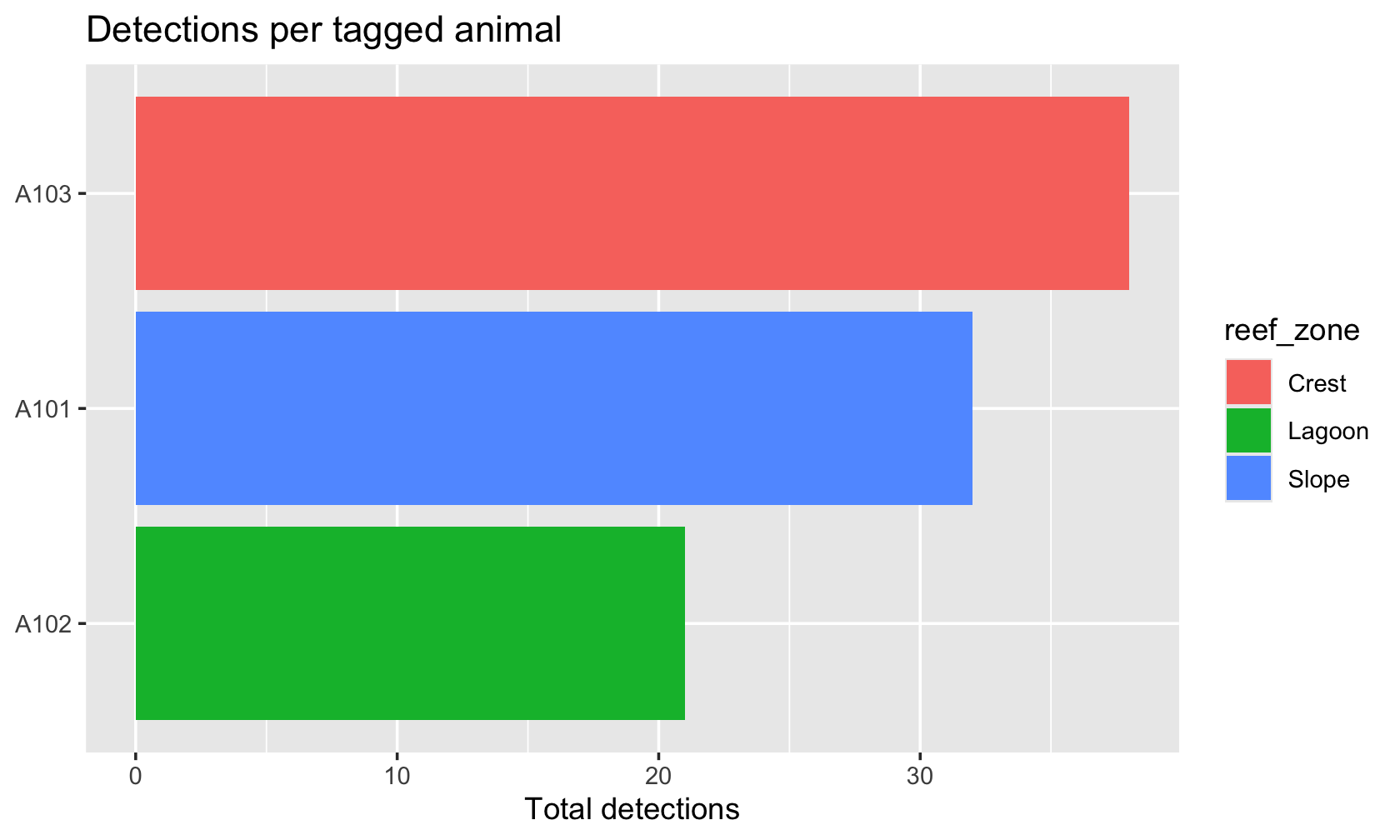

Go deeper (open access)

These quests are a short path; the field already publishes free courses, scripts, and books. We paraphrase their goals below—follow the links for full material.

Core R & reproducible workflows

The Carpentries — Programming with R teaches modular analysis with loops and functions using worked examples—not every R function, but habits that match our Base R quests (Software Carpentry, CC BY).
R for Reproducible Scientific Analysis (Carpentries) extends that to multi-step, reproducible pipelines—close to how we chain dplyr and save scripts in RStudio.
R for Data Science (2e) (Wickham, Çetinkaya-Rundel, Grolemund) is the standard free book for import → tidy → transform → plot; our dplyr track follows the same verb order (CC BY-NC-ND).
Advanced R (Wickham) explains why R behaves like a functional language and how map-style thinking fits data analysis—background for our purrr track.

Marine & ecological statistics (people & labs)

Seascape Models — Chris Brown (University of Tasmania) shares open teaching on predictive ecological modelling in R, with course notes and data on GitHub—quantitative marine decision-making with reproducible scripts.
Statistics for ecologists (Master course) (Gimenez) — slides, practicals, and R code under CC BY 4.0; strong on GLMMs and Bayesian ideas used in capture–recapture and population ecology.
Bayesian Data Analysis in Ecology (Korner-Nievergelt et al.) — free, evolving e-book with R/Stan examples; useful once regression and purrr-style replication make sense.
R Workshops @ UQ — long-running workshops from mathematical ecologists at the University of Queensland on R and applied modelling for researchers (SCIE3360 also stresses reproducible data science in R for life and environmental sciences).

Universities & field training (context, not enrollment)

University of St Andrews Statistical Ecology MSc and incoming MSc guidance treat R as assumed tooling for modern applied statistics; CREEM runs structured stats training for St Andrews researchers.
University of Plymouth embeds statistics workshops in marine biology field courses and points students to R-focused texts via library guides (e.g. biologist-oriented R and reproducible research titles).
Max Planck Institute of Animal Behavior — AniMove runs open-source–focused training on movement, remote sensing, and R; recorded material is linked from Movebank teaching.
FIU — Simon Dedman’s open graduate stats / R materials cover tidying, SDMs, and causal modelling on marine datasets (see also reproducible reef analyses on Zenodo).
Galápagos — the Charles Darwin Foundation has run free community courses on statistics and R with local partners; the Galapagos Science Center supports interdisciplinary, data-heavy conservation research.

Functional tools (packages & references)

purrr (Henry & Wickham) — official reference for typed map functions used in our Intermediate purrr track.
data.table — documentation and vignettes for [i, j, by] syntax in our Advanced track.
Big Book of R — curated chapters linking base R, tidyverse, and workflow topics; handy index when you outgrow quests.

Self-paced ecology coding

Coding Club — Data Science for Ecologists (University of Edinburgh) — free, self-paced R tutorials and quizzes aimed at environmental scientists; good parallel practice alongside any quest level.

If you use AI tools while learning, treat these sources as the ground truth: run their code, compare output to ours, and cite them when you adapt their workflows.

Functional programming · Beginner (Base R)

Q1 · Vectors, names, and types

Q2 · Subsetting [, $, [[

Q3 · if, else, and ifelse

Q4 · for loops on real rows

Q5 · Writing functions

Q6 · apply() on fisheries matrix

Q7 · lapply() lists

Q8 · sapply() simplification traps

Q9 · vapply() safe types

Q10 · split() + lapply()

Q11 · tapply() group means

Q12 · aggregate() classic

Q13 · mapply() paired vectors

Q14 · set.seed() & sample()

Q15 · order() and sorting logic

Q16 · unique() & table()

Q17 · str(), class(), debugging

Q18 · Nested if-else for QC

Q19 · Loop vs vectorised choice

Q20 · Base R mini-capstone

Go deeper (open access)

Core R & reproducible workflows

Marine & ecological statistics (people & labs)

Universities & field training (context, not enrollment)

Functional tools (packages & references)

Self-paced ecology coding

Q2 · Subsetting `[`, `$`, `[[`