Functional programming · Intermediate (purrr & furrr)

Intermediate · purrr
Author

Pablo Fuenzalida

Published

July 21, 2026

Functional programming · Intermediate (purrr & furrr)

Lists and map for tags, bursts, years. Do Base R + dplyr first.

Q1 · Lists as ecology objects

An R list holds heterogeneous objects — data frames, vectors, metadata — in one named container.

by_site <- split(reef, reef$site) # base split to named list
class(by_site) # should be 'list'
[1] "list"
names(by_site) # site names as list names
[1] "East"  "North" "South"
lapply(by_site, nrow) # rows per site
$East
[1] 20

$North
[1] 20

$South
[1] 20

Q2 · map() intuition

map() applies a function to each list element and returns a list of results — always, unlike the sapply() simplification surprises in base R.

species_lists <- map(by_site, ~ unique(.x$species)) # .x is each site df
species_lists # list of character vectors
$East
[1] "Parrotfish"  "Surgeonfish" "Grouper"     "Snapper"     "Damselfish" 

$North
[1] "Parrotfish"  "Surgeonfish" "Grouper"     "Snapper"     "Damselfish" 

$South
[1] "Parrotfish"  "Surgeonfish" "Grouper"     "Snapper"     "Damselfish" 
lengths(species_lists) # how many species per site
 East North South 
    5     5     5 

Also:

by_port <- split(fishery, fishery$port)
map_int(by_port, nrow)
    Broome     Cairns Mooloolaba 
         9          9          6 

Also:

by_zone <- split(acoustic, acoustic$reef_zone)
map_chr(by_zone, ~ .x$receiver[1])
 Crest Lagoon  Slope 
  "R2"   "R9"  "R11" 

Q3 · map_dbl(), map_chr()

Typed maps map_dbl(), map_int(), map_chr() assert return types — the purrr analogue of vapply() from Level 1.

mean_counts <- map_dbl(by_site, ~ mean(.x$count)) # numeric vector out
mean_counts # named by site
 East North South 
10.95  8.80  9.80 
sum(mean_counts) # sanity check total
[1] 29.55

Q4 · map2() paired columns

map2() walks two parallel vectors element-wise — year paired with species, depth paired with pitch.

labels <- map2_chr(fishery$year, fishery$species, ~ paste(.x, .y, sep = "-"))
head(labels) # first few composite ids
[1] "2018-Snapper" "2018-Grouper" "2018-Tuna"    "2018-Shark"   "2019-Snapper"
[6] "2019-Grouper"
length(labels) == nrow(fishery) # lengths must match
[1] TRUE

Also:

map2_dbl(reef$count, reef$depth_m, function(c, d) if (d > 0) c / d else NA_real_)[1:5]
[1] 0.6451613 1.9354839 0.1612903 1.1290323 3.3870968

Also:

b1 <- biolog[biolog$burst_id == 1, ]
map2_dbl(b1$depth_m[-length(b1$depth_m)], b1$depth_m[-1], ~ .y - .x)[1:5]
[1]  0.26751027 -0.31068411 -0.02501225 -0.06485909  0.20001095

Q5 · pmap() row-wise

pmap() maps over rows of a data frame — row-wise logic without an explicit index i.

ac5 <- acoustic |> dplyr::slice_head(n = 5) # tiny slice
summaries <- pmap_chr(ac5, function(animal_id, receiver, detections, reef_zone) {
  paste0(animal_id, " @ ", receiver, ": ", detections, " (", reef_zone, ")")
})
summaries # one string per row
[1] "A101 @ R11: 5 (Slope)" "A101 @ R2: 2 (Crest)"  "A101 @ R6: 7 (Slope)" 
[4] "A101 @ R1: 4 (Crest)"  "A101 @ R5: 5 (Slope)" 

Also:

r3 <- reef |> slice_head(n = 3)
pmap_chr(r3, function(transect_id, site, species, count, depth_m) {
  paste0(transect_id, " ", species, ": ", count, " @ ", site)
})
[1] "T01 Parrotfish: 4 @ North"   "T01 Surgeonfish: 12 @ North"
[3] "T01 Grouper: 1 @ North"     

Also:

f3 <- fishery |> slice_head(n = 3)
pmap_chr(f3, function(year, species, tonnes, port) paste0(year, " ", species, " ", tonnes, "t @ ", port))
[1] "2018 Snapper 75.7t @ Cairns"     "2018 Grouper 79.6t @ Mooloolaba"
[3] "2018 Tuna 23.5t @ Broome"       

Q6 · map_dfr() simulations

map_dfr() row-binds data frame results — ideal for simulation replicates or per-group outputs.

set.seed(7) # reproducible draws
sp <- unique(reef$species) # species labels
sim <- map_dfr(sp, function(s) { # one df per species
  tibble(species = s, draw = rpois(3, lambda = 5)) # three random counts
})
sim # stacked draws
# A tibble: 15 × 2
   species      draw
   <chr>       <int>
 1 Parrotfish     11
 2 Parrotfish      4
 3 Parrotfish      2
 4 Surgeonfish     2
 5 Surgeonfish     3
 6 Surgeonfish     7
 7 Grouper         4
 8 Grouper        10
 9 Grouper         3
10 Snapper         5
11 Snapper         3
12 Snapper         3
13 Damselfish      7
14 Damselfish      2
15 Damselfish      5

Also:

ports <- unique(fishery$port)
map_dfr(ports, function(p) {
  tibble(port = p, tonnes = runif(3, 20, 90))
})
# A tibble: 9 × 2
  port       tonnes
  <chr>       <dbl>
1 Cairns       25.9
2 Cairns       59.2
3 Cairns       20.6
4 Mooloolaba   89.0
5 Mooloolaba   42.2
6 Mooloolaba   64.8
7 Broome       40.7
8 Broome       89.8
9 Broome       83.4

Also:

rx <- unique(acoustic$receiver)[1:4]
map_dfr(rx, function(r) tibble(receiver = r, sim_det = rpois(3, lambda = 4)))
# A tibble: 12 × 2
   receiver sim_det
   <chr>      <int>
 1 R11            9
 2 R11            1
 3 R11            4
 4 R2             4
 5 R2             8
 6 R2             3
 7 R6             5
 8 R6             3
 9 R6             2
10 R1             2
11 R1             3
12 R1             6

Q7 · safely() errors as data

safely() wraps a function to return result or error instead of stopping — essential on messy field spreadsheets.

raw <- c("12", "4.5", "NA", "oops") # mixed strings
parsed <- map(raw, safely(as.numeric)) # list of result/error
ok <- map_lgl(parsed, ~ is.null(.x$error)) # which succeeded
map_dbl(parsed[ok], "result") # extract numeric successes
[1] 12.0  4.5   NA   NA

Also:

raw_counts <- c("8", "12", "12a", "3")
map(raw_counts, safely(as.numeric))
[[1]]
[[1]]$result
[1] 8

[[1]]$error
NULL


[[2]]
[[2]]$result
[1] 12

[[2]]$error
NULL


[[3]]
[[3]]$result
[1] NA

[[3]]$error
NULL


[[4]]
[[4]]$result
[1] 3

[[4]]$error
NULL

Also:

raw_t <- c("45.2", "", "88")
map(raw_t, safely(as.numeric))
[[1]]
[[1]]$result
[1] 45.2

[[1]]$error
NULL


[[2]]
[[2]]$result
[1] NA

[[2]]$error
NULL


[[3]]
[[3]]$result
[1] 88

[[3]]$error
NULL

Q8 · walk() side effects

walk() maps for side effects such as messages or file writes and discards return values.

walk(names(by_site), function(nm) { # iterate site names
  message("Site: ", nm, " — rows: ", nrow(by_site[[nm]])) # logging side effect
})
invisible(NULL) # walk returns input invisibly

Q9 · reduce() combine lists

reduce() folds a list with a binary function — combine vectors or merge tables stepwise.

by_an <- split(acoustic$detections, acoustic$animal_id) # list of nums
per_an <- map_dbl(by_an, sum) # one total per animal tag
total_det <- reduce(per_an, `+`) # fold scalar sums together
total_det # grand total detections
[1] 91

Q10 · list-columns intro

Tibbles can store list-columns — each cell holds a vector or mini data frame before unnest().

nested_bio <- biolog |> # biologging table
  group_by(burst_id) |> # one row per burst soon
  summarise(times = list(seconds), depths = list(depth_m), .groups = "drop")
nested_bio # list-columns visible
# A tibble: 10 × 3
   burst_id times      depths    
      <int> <list>     <list>    
 1        1 <int [20]> <dbl [20]>
 2        2 <int [20]> <dbl [20]>
 3        3 <int [20]> <dbl [20]>
 4        4 <int [20]> <dbl [20]>
 5        5 <int [20]> <dbl [20]>
 6        6 <int [20]> <dbl [20]>
 7        7 <int [20]> <dbl [20]>
 8        8 <int [20]> <dbl [20]>
 9        9 <int [20]> <dbl [20]>
10       10 <int [20]> <dbl [20]>
nested_bio$depths[[1]] # first burst depth vector
 [1] 4.798260 5.065770 4.755086 4.730074 4.665214 4.865225 5.037666 5.419779
 [9] 5.008206 5.065953 5.231723 5.179684 5.222335 5.230477 4.876622 5.201536
[17] 4.637366 4.143637 3.940643 4.300171

Q11 · map on telemetry splits

Split acoustic data by animal_id, map summaries — the animal-centric pattern in movement ecology.

by_animal <- group_split(acoustic, animal_id) # list of tibbles
max_det <- map_dbl(by_animal, ~ max(.x$detections)) # peak ping count
names(max_det) <- map_chr(by_animal, ~ unique(.x$animal_id)) # name elements
max_det # per-tag max
A101 A102 A103 
   7    5    7 

Q12 · map on fishery years

Split fishery by year and map total tonnes — functional annual report tables.

by_year <- group_split(fishery, year) # one df per year
year_tot <- map_dbl(by_year, ~ sum(.x$tonnes)) # annual totals
setNames(year_tot, map_int(by_year, ~ unique(.x$year))) # names = years
 2018  2019  2020  2021  2022  2023 
246.5 277.1 301.1 241.6 202.5 179.8 
year_tot # numeric summary
[1] 246.5 277.1 301.1 241.6 202.5 179.8

Q13 · map2 weights & counts

map2() on paired vectors supports weighted calculations — tonnes times price, detections times effort.

x <- biolog$depth_m[1:10] # depths subsample
w <- rep(1, 10) # equal weights demo
weighted <- map2_dbl(x, w, ~ .x * .y) # element products
sum(weighted) / sum(w) # weighted mean depth
[1] 4.941123

Q14 · possibly() softer failures

possibly() replaces errors with a default value — softer than safely() when you want NA back.

mult <- c(1, 2, 0, 4) # includes zero divisor
safe_div <- possibly(function(a, b) a / b, otherwise = NA_real_)
map2_dbl(acoustic$detections[1:4], mult, safe_div) # NA where divide fails
[1]   5   1 Inf   1

Q15 · quietly() hide messages

quietly() captures messages while returning results — useful when mapped functions are chatty.

chatty_mean <- function(x) { # function with message
  message("computing mean on length ", length(x))
  mean(x)
}
q <- quietly(chatty_mean) # wrap to capture noise
res <- map(by_site, ~ q(.x$count)) # list of quiet results
map_dbl(res, "result") # extract means only
 East North South 
10.95  8.80  9.80 

Q16 · furrr parallel map

furrr future_map() mirrors map() on parallel workers — worth it on heavy simulations, not tiny reef tables.

has_furrr <- requireNamespace("furrr", quietly = TRUE) # check package
if (has_furrr) {
  suppressPackageStartupMessages({ library(furrr); library(future) })
  plan(multisession, workers = 2) # local worker pool
  future_map_dbl(by_site, ~ mean(.x$count)) # parallel map
} else {
  message("Install furrr for parallel demo; using map_dbl")
  map_dbl(by_site, ~ mean(.x$count)) # serial fallback
}
 East North South 
10.95  8.80  9.80 

Q17 · future plans & workers

The future plan() selects sequential vs multisession execution — set once before furrr maps.

time_serial <- system.time({ # time serial map
  map_dbl(by_site, ~ mean(.x$count))
})
time_serial # print timing object
   user  system elapsed 
  0.001   0.000   0.000 

Q18 · map deep on biologging

Map over burst splits to build hierarchical summaries — ‘deep’ mapping across nested structure.

burst_stats <- biolog |> # biologging data
  group_split(burst_id) |> # list of burst tibbles
  map(~ summarise(.x, mean_depth = mean(depth_m), n_sec = n()))
burst_tbl <- map_dfr(burst_stats, identity) # row-bind summaries
head(burst_tbl) # one row per burst
# A tibble: 6 × 2
  mean_depth n_sec
       <dbl> <int>
1       4.87    20
2       4.43    20
3       4.76    20
4       5.57    20
5       5.26    20
6       4.98    20

Q19 · compose functions

compose() builds function pipelines — conceptual kin to |> but for function values passed to map.

scale01 <- function(x) (x - min(x)) / (max(x) - min(x)) # min-max scale
round2 <- function(x) round(x, 2) # two decimals
fmt <- compose(round2, scale01) # combined function
fmt(fishery$tonnes) # formatted vector
 [1] 0.47 0.50 0.07 0.41 0.34 0.51 0.30 0.55 1.00 0.07 0.23 0.58 0.64 0.46 0.00
[16] 0.32 0.27 0.10 0.20 0.56 0.34 0.26 0.12 0.24

Q20 · purrr capstone

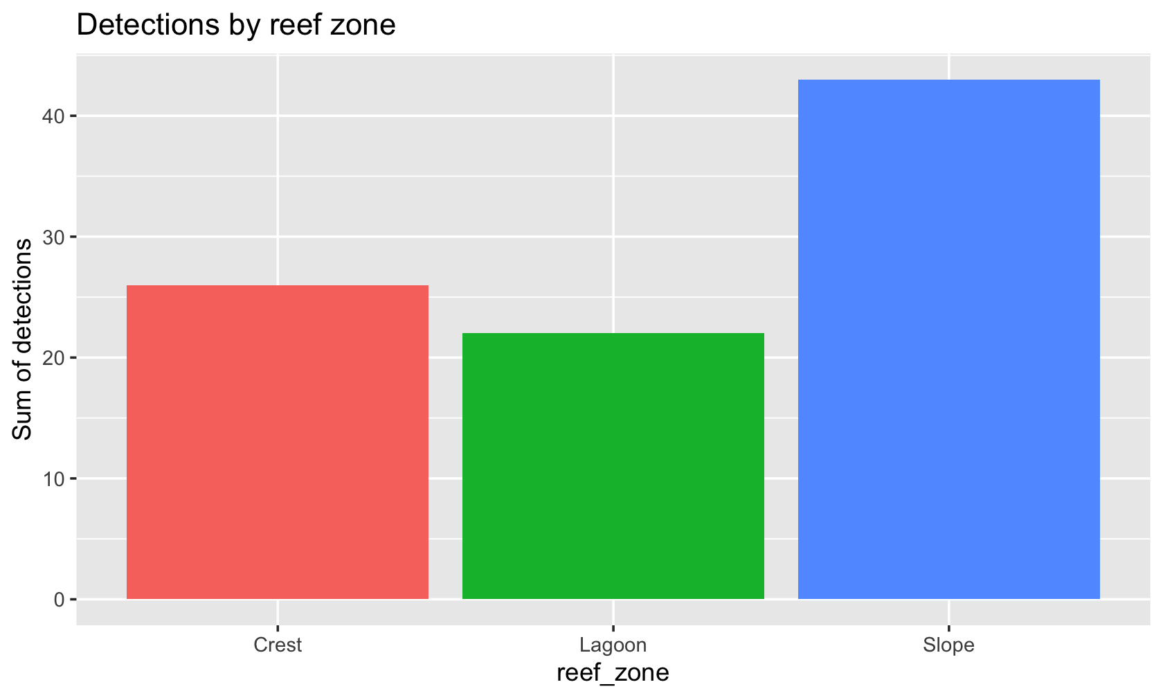
Integrate split, map, and map_dfr() on acoustic data — the workflow to verify before batch-processing receiver exports with AI.

zone_list <- group_split(acoustic, reef_zone) # list by habitat zone
zone_summary <- map_dfr(zone_list, function(df) {
  tibble(
    reef_zone = unique(df$reef_zone),
    total_det = sum(df$detections),
    n_rows = nrow(df)
  )
})
ggplot(zone_summary, aes(x = reef_zone, y = total_det, fill = reef_zone)) +
  geom_col(show.legend = FALSE) + # bar chart by zone
  labs(title = "Detections by reef zone", y = "Sum of detections")