library(tidyverse)   # data wrangling / manipulación de datos
library(units)       # unit conversion / conversión de unidades
library(lubridate)   # date-time handling / manejo de fechas y horas
library(plotly)      # interactive plots / gráficos interactivos
library(zoo)         # rolling functions / funciones deslizantes
library(signal)      # Butterworth filter / filtro Butterworth
library(tagtools)    # tag-specific functions (njerk, detect_peaks, fix_pressure) / funciones específicas para tags
library(janitor)     # clean column names / limpiar nombres de columnas
library(purrr)       # functional mapping / mapeo funcional
library(furrr)       # parallel mapping / mapeo paralelo
library(future) # parallel backend / backend paraleloRorqual whale biomechanics with kinematic data
Written in both English and Spanish 🇬🇧🇪🇸 — every section appears in both languages | Escrito en inglés y español 🇬🇧🇪🇸 — cada sección aparece en ambos idiomas
biologger
high resolution
biomechanics
A bilingual (English & Spanish) workflow for detecting lunge-feeding events in fin whales from high-resolution CATS bio-logger data. | Un flujo de trabajo bilingüe (inglés y español) para detectar embestidas de alimentación en ballenas de aleta a partir de datos de biologgers CATS de alta resolución.
Overview | Resumen
Hi! This workflow processes high-resolution bio-logging tag data from fin whales (Balaenoptera physalus) to detect lunge-feeding events. It combines data from CATs cameras (customr animal tracking solutions; cats.is), which record tri-axial accelerometer and gyroscope (roll) data, applies kinematic filters, and produces annotated depth profiles with predicted lunges. In this workflow, we smooth our kinematic data, convert it to jerks, find peaks in those jerks then filter using roll and depth to ensure we reduce the amount of false positives in the output.
Holi mi amorictas. Este flujo de trabajo procesa datos de los marcas biologgers, especificamente el marca CATs (solutiones de marcado animals cats.is) en alta resolución de biotelemétría de los ballenas fin / aleta (Balaenoptera physalus) para detectar eventos de alimentación por embestida. Combina datos de acelerómetro triaxial y giroscopio (balanceo), aplica filtros cinemáticos y produce perfiles de profundidad anotados con embestidas predichas.
1. Libraries | Packetes
2. Import Raw Data | Importar datos crudo
# import a single deployment at a time
# solol importad una deployment cada vez por este analysis
dat <- read_csv("20220128-174624-dep1.csv",
                col_types = cols(`Time (UTC)` = col_time(),
                                 `Time (local)` = col_time()))
dat <- dat %>%
  janitor::clean_names() # standardise column structures / estandarizar estructura de columnas
3. Clean & Format | Limpiar y formatear
dat1 <- dat %>%
  rename(depth = depth_100bar_m,
         temperature = temperature_depth_c) %>%
  dplyr::select(1, 2, 5:10, temperature, depth) %>%  # keep relevant columns / conservar columnas relevantes
  mutate( # lubridate to change date format structures within columns
    date_utc      = dmy(date_utc),
    datetime_utc  = as_datetime(paste(date_utc, time_utc), tz = "UTC"),
    datetime      = with_tz(datetime_utc, tzone = "America/Santiago"), # convert to Chilean time / convertir a hora chilena
    time          = hms::as_hms(format(datetime, "%H:%M:%S"))
  ) %>%
  dplyr::select(datetime, time, everything(), -date_utc, -time_utc, -datetime_utc)

str(dat1)
4. Filter to deployment Window | Filtrar a la ventana de deployment
EN: In this step, we use plotly to make an interactive plot to cut the data to when the tag was deployed on the animal, and when it fell off. You can do this statically, by plotting a depth plot, and just finding the minute or so before it was placed onthe animal, and a bit after
ES: En este numero, voy a filtrar sus datos solo para tener el tiempo con la marca en el animal. Te vas a discubera donde puedes cortar con una plot de profundidad interactiva (plotly) o estatica (ggplot), y miera donde entrar sus datos de buceando, y donde terminar.
first_cut <- ymd_hms("2022-01-27 15:31:00", tz = tz(dat1$datetime)) # deployment start / inicio de marca
last_cut  <- ymd_hms("2022-01-28 02:11:00", tz = tz(dat1$datetime)) # tag fell off / el marca se fui arriba

dat2 <- dat1 %>%  # filter data to 1 min before and after the annotations
  dplyr::filter(datetime >= first_cut & datetime <= last_cut) # cut to tag time window / recortar a ventana de forrajeo diurno

ggplot(dat2 %>% # static plot to check (plot estatico para mierar)
         mutate(second = floor_date(datetime, "second")) %>%
         group_by(second) %>%
         slice_head(n = 1), # downsample to 1 Hz for display / reducir a 1 Hz para visualización
       aes(x = datetime, y = depth)) +
  geom_line() +
  scale_y_reverse()
5. Convert Gyroscope Units | Convertir unidades del giroscopio
EN: Gyroscope values are recorded in milliradians per second (mrad/s). We convert to degrees per second (deg/s) following methods by Goldbogen et al. (2006), as degrees are more interpretable. Values are normalised to the -180° to +180° range.
ES: Los valores del giroscopio se registran en miliradianes por segundo (mrad/s). Los convertimos a grados por segundo (deg/s) siguiendo a métodos de Goldbogen et al. (2006), ya que los grados son más interpretables. Los valores se normalizan al rango -180° a +180°.
dat3 <- dat2 %>%
  mutate(across(ends_with("_mrad_s"), ~ .x * 0.001, .names = "{.col}_to_rad_s")) %>%   # mrad/s → rad/s
  mutate(across(ends_with("_to_rad_s"),
                list(deg_s = ~ as.numeric(set_units(as_units(.x, "radians"), "degrees"))))) %>%  # rad/s → deg/s
  mutate(across(ends_with("_deg_s"), ~ (.x + 180) %% 360 - 180)) %>%                   # normalise to ±180° / normalizar a ±180°
  rename_with(~ str_replace(.x, "_mrad_s_to_rad_s_deg_s", "_deg_s"), ends_with("_deg_s")) %>%
  dplyr::select(datetime, time, accelerometer_x_m_s, accelerometer_y_m_s,
                accelerometer_z_m_s, matches("gyroscope_._deg_s"), temperature, depth)

summary(dat3[, grep("gyroscope", names(dat3))]) # sanity check / verificación
6. Compute Kinematic Magnitudes | Calcular magnitudes cinemáticas
EN: This step is to compute the magnitude of acceleration, across all three axis’. We do this using methods similar to previous studies such as Cade et al., 2016; calculating forward speed from tag jiggle. This is dependant on the sample scale of the data, if its sample is not 10hz per second, you will need to edit this to whichever hz your data is sampled at.
ES: Este paso consiste en calcular la magnitud de la aceleración a lo largo de los tres ejes. Lo hacemos utilizando métodos similares a estudios previos como Cade et al., 2016; Calculando la velocidad hacia adelante a partir del movimiento de la etiqueta. Esto depende de la escala de muestra de los datos; si la muestra no es de 10 Hz por segundo, tendrás que editarlo a la frecuencia en la que se muestren tus datos.
dat4 <- dat3 %>%
  mutate(
    mag_acceleration = sqrt(accelerometer_x_m_s^2 + accelerometer_y_m_s^2 + accelerometer_z_m_s^2), # Euclidean norm / norma euclidiana
    mag_gyroscope    = sqrt(gyroscope_x_deg_s^2 + gyroscope_y_deg_s^2 + gyroscope_z_deg_s^2),
    seconds          = row_number() / 10,   # elapsed seconds at 10 Hz / segundos transcurridos a 10 Hz
    minutes          = row_number() / 600   # elapsed minutes / minutos transcurridos
  )

head(dat4) # como vas ? How is our data?
7. Correct Depth (Pressure) | Corregir profundidad (presión)
EN: We use the wonderful package of tagtools, from Stacey DeGruiter et al., to ensure that 0 in depth, is a true 0. A problem tags that dive to depth encounter is having a false middle point of zero, due to the pressure sensor within the biologger being slighlty off in calculating ambient pressure. This may mean your depth data and dives are not truly starting / ending close to the surface, but maybe 5 metres deep or above the surface instead. Due to the fact we will be using a 2 metre depth filter, we need to ensure depth is corrected as much as possible. Luckily, tagtools::fix_pressure does all the work for us.
Just as a note, I’ve played with this function quite a bit, and even when data are sampled at 10 - 50hz, this only seems to work when you input the sampling rate as 5. However, you as a researcher are encouraged to explore this problem yourself to see which approach works best, and decide the most appropriate approach.
ES: Usamos el maravilloso paquete de herramientas de etiquetas, de Stacey DeGruiter et al., para asegurarnos de que 0 en profundidad sea un 0 verdadero. Un problema de etiquetas que se adentran en profundidad es tener un falso punto medio cero, debido a que el sensor de presión dentro del biológico está ligeramente desviado al calcular la presión ambiente. Esto puede significar que tus datos de profundidad y las inmersiones no empiezan o terminan realmente cerca de la superficie, sino quizá a 5 metros de profundidad o por encima de la superficie. Debido a que vamos a usar un filtro de 2 metros de profundidad, debemos asegurarnos de corregir la profundidad tanto como sea posible. Por suerte, tagtools::fix_pressure hace todo el trabajo por nosotros.
Una nota media importante, he probado bastante esta función, y aunque los datos se muestrean a 10 - 50hz, esto solo parece funcionar cuando introduces la frecuencia de muestreo como 5. Sin embargo, como investigador se te anima a explorar este problema por ti mismo para ver cuál enfoque funciona mejor y decidir el más adecuado.
adepth <- tagtools::fix_pressure(p = dat4$depth, # depth data
                                 t = dat4$temperature, #temperature data
                                       sampling_rate = 5,  # sample rate
                                       maxp = 0.0001) # max depth for which the animal could be at the surface, also play with this value

dat4$depth <- adepth$p # replace raw depth with corrected values / reemplazar profundidad bruta con valores corregidos

plot_ly(data = data.frame(time = seq_along(adepth$p) / 600, depth = adepth$p),
        x = ~time, y = ~depth) %>%
  add_lines() %>%
  layout(yaxis = list(autorange = "reversed", title = "Depth (m)"),
         xaxis = list(title = "Minutes"))
8. Smooth Accelerometer & Roll Data (Butterworth Band-Pass Filter) | Suavizar datos de acelerómetro y balanceo (Filtro Butterworth pasa-banda)
EN: Attaching a tag to an animal does not give us direct forward speed, a trouble many have encountered. Which means, we have to estimate it, from our acceleration data. Luckily, a bunch of smart Stanford people have done that already; Cade et al., 2018 Estimating forward speed from tag jiggle.
We have calculated the magnitude of acceleration already, which gives us acceleration across all three axis we have; x, y and z. From this data, we have a LOT of noise, making it hard for us to tease apart important events such as lunges with simple movements we aren’t interested in.
High-frequency “jiggle” — small vibrations from tag movement in the water column — contaminates the raw accelerometer signal. We will smoothen these messy data out. A band-pass Butterworth filter isolates the biologically meaningful frequency band (1–4 Hz here) and removes both slow tag drift (< 1 Hz) and high-frequency noise or tag jiggle (> 4 Hz). We use nyquitist frequency to decide our band pass location and width in hz, so you must also do so by obeying this rule if your sample rate is different to 10 hz (similar to Cade et al., 2018; they used a high-pass filter instead of band-pass, but suggested both can work). For example, if it is 50 hz sample rate, as some of our data is, we shall expand the band from 1 - 4 hz to 10 - 24 hz, to be under half (25), and above the lower end (9 and under).
We then apply Root Mean Square (RMS) smoothing with 0.5-second bins (Cade et al., 2018). This bin size should not disrupt our ability to detect what we are attempting, as this biological behaviour occurs over 2 - 8 seconds in its duration (Cade et al., 2016), leaving plenty of time for our product to detect a signal. The same filter is applied to gyroscope x to create a smoothed roll product it for the lunge-detection step.
ES: Colocar una etiqueta en un animal no nos da velocidad directa hacia adelante, un problema que muchos han encontrado. Lo que significa que tenemos que estimarlo a partir de nuestros datos de aceleración. Por suerte, un montón de gente lista de Stanford ya lo ha hecho; Cade et al., 2018 Estimación de la velocidad hacia adelante a partir del movimiento de etiqueta.
Ya hemos calculado la magnitud de la aceleración, lo que nos da aceleración a lo largo de los tres ejes que tenemos; X, Y y Z. A partir de estos datos, tenemos tanto ruido, lo que dificulta distinguir eventos importantes como las embestidas con movimientos simples que no nos interesan.
El “tambaleo” de alta frecuencia —pequeñas vibraciones derivadas del movimiento de la etiqueta en la columna de agua— contamina la señal cruda del acelerómetro. Vamos a suavizar estos datos confusos. Un filtro Butterworth pasa banda aísla la banda de frecuencia biológicamente significativa (1–4 Hz aquí) y elimina tanto l a deriva lenta de la etiqueta (4 Hz). Usamos la frecuencia nyquitist para decidir la ubicación y ancho de la banda pasa en Hz, así que también debes hacerlo obedeciendo esta regla si tu frecuencia de muestreo es diferente a la de 10 Hz (similar a Cade et al., 2018; usaron un filtro pasa altos en lugar de pasa banda, pero sugirieron que ambos pueden funcionar). Por ejemplo, si es una frecuencia de muestreo de 50 Hz, como ocurre con algunos de nuestros datos, ampliaremos la banda de 1 a 4 Hz a 10 - 24 Hz, para que esté por debajo de la mitad (25) y por encima del extremo inferior (9 o menos).
Luego aplicamos suavizado de cuadrado medio raíz (RMS) con contenedores de 0,5 segundos (Cade et al., 2018). Este tamaño de contenedor no debería interrumpir nuestra capacidad para detectar lo que intentamos, ya que este comportamiento biológico ocurre durante 2 - 8 segundos en su duración (Cade et al., 2016), dejando tiempo suficiente para que nuestro producto detecte una señal. El mismo filtro se aplica al giroscopio x para crear un producto de rodeo suavizado para el paso de detección de zancadas.
fs        <- 10   # sampling rate in Hz / frecuencia de muestreo en Hz
bin_width <- 0.5  # RMS bin width in seconds / ancho de ventana RMS en segundos
low_cut   <- 1    # lower frequency cutoff (Hz) / límite inferior de frecuencia (Hz)
high_cut  <- 4    # upper frequency cutoff (Hz); must be < fs/2 / límite superior (Hz); debe ser < fs/2

bp_filt <- butter(4, c(low_cut, high_cut) / (fs / 2), type = "pass") # 4th-order Butterworth / Butterworth de orden 4

dat4$accel_bp <- filtfilt(bp_filt, dat4$mag_acceleration) # zero-phase filter acceleration / filtro de fase cero en aceleración
dat4$roll_bp  <- filtfilt(bp_filt, dat4$gyroscope_x_deg_s) # zero-phase filter roll / filtro de fase cero en balanceo

dat5 <- dat4 %>%
  mutate(bin = floor(seconds / bin_width)) # assign each sample to a 0.5s bin / asignar cada muestra a una ventana de 0,5 s

rms_by_bin <- dat5 %>%
  group_by(bin) %>%
  summarise(
    accel_rms_bp = sqrt(mean(accel_bp^2, na.rm = TRUE)), # RMS of band-passed acceleration / RMS de aceleración filtrada
    roll_rms_bp  = sqrt(mean(roll_bp^2,  na.rm = TRUE))  # RMS of band-passed roll / RMS de balanceo filtrado
  )

dat6 <- dat5 %>%
  left_join(rms_by_bin, by = "bin") %>%  # join both dataframes together
  dplyr::select(-bin)

str(dat6) # how is our data looking ? Mirar su datos
9. Compute Jerk & Detect Peaks | Calcular jerk y detectar Cumbres
EN: Jerk is the time derivative of acceleration — it measures how rapidly acceleration changes between consecutive samples. Peaks in jerk coincide with the abrupt body movements characteristic of lunge events in rorqual whales. We compute jerk on the RMS-smoothed acceleration, then use tagtools::detect_peaks() to find local maxima above a chosen threshold (Sweeney et al., 2019).
ES: Jerk (tirón) es la derivada temporal de la aceleración — mide qué tan rápido cambia la aceleración entre muestras consecutivas. Los cumbres de jerk coinciden con los movimientos corporales abruptos característicos de las embestidas en ballenas rorcuales. Calculamos el jerk sobre la aceleración suavizada por RMS, luego usamos tagtools::detect_peaks() para encontrar máximos locales por encima de un umbral elegido (Sweeney et al., 2019).
dat6$jerk <- tagtools::njerk(as.matrix(dplyr::select(dat6,
                                                     accel_rms_bp)), # use a matrix of acceleration to calculate jerk
                                          sampling_rate = 10) # normalised jerk / jerk normalizado
dat6$jerk[is.na(dat6$jerk)] <- 0 # replace NAs with 0 / reemplazar NAs en los bordes

pks <- tagtools::detect_peaks(dat6$jerk, sr = 10, thresh = 2,
                               plot_peaks = FALSE, bktime = 10) %>%  # bktime = min. time between peaks (s) / tiempo mínimo entre cumbres (s)
  mutate(peak_seconds = peak_time / 10) # convert sample index to seconds / convertir índice de muestra a segundos

dat7 <- dat6 %>%
  mutate(jerk_peak = if_else(round(seconds, 2) %in% round(pks$peak_seconds, 2), 1L, 0L)) # flag peak samples / marcar muestras de cumbres

ggplot(dat7, aes(x = datetime, y = depth)) + # plot it
  geom_line(colour = "grey50") + # to check it worked
  scale_y_reverse() + # and is in the correct places in your dive profile
  geom_point(data = dplyr::filter(dat7, jerk_peak == 1),
             aes(x = datetime, y = depth), colour = "red", size = 2, shape = 4) +
  labs(x = "Time | Tiempo", y = "Depth (m) | Profundidad (m)",
       title = "Jerk peaks | cumbres de jerk") +
  theme_minimal()
10. Filter Peaks Using Roll | Filtrar cumbres usando balanceo
EN: Not all acceleration peaks are lunges — surface breaths and other behavioural events (Goldbogen et al., 2013) also produce acceleration spikes. Lunges are characterised by body rolling: the whale rolls laterally as it engulfs prey. The roll_filter() function examines a ± time_window second window around each jerk peak and checks whether the smoothed roll rate exceeds gyro_threshold (deg/s) for at least min_duration consecutive seconds. Peaks that do not meet this roll criterion are removed, eliminating most breath events. A depth threshold (≥ 2 m) is applied afterwards to remove any remaining surface artefacts.
ES: No todos los cumbres de aceleración son embestidas — las respiraciones superficiales también producen cumbres de aceleración. Las embestidas se caracterizan por el balanceo corporal: la ballena se balancea lateralmente al engullir presas. La función roll_filter() examina una ventana de ±time_window segundos alrededor de cada pico de jerk y verifica si la tasa de balanceo suavizada supera gyro_threshold (deg/s) durante al menos min_duration segundos consecutivos. Los cumbres que no cumplen este criterio de balanceo se eliminan, eliminando la mayoría de los eventos de respiración. Luego se aplica un umbral de profundidad (≥ 2 m) para eliminar artefactossuperficiales restantes.
roll_filter <- function(dat, gyro_col, gyro_threshold, time_window, min_duration, fs,
                        parallel = FALSE) {
  peaks      <- dplyr::filter(dat, jerk_peak == 1)
  all_times  <- dat$seconds
  all_gyro   <- dat[[gyro_col]]
  n_consec   <- ceiling(min_duration * fs) # minimum consecutive samples above threshold / muestras consecutivas mínimas sobre el umbral
  .map_func  <- if (parallel) furrr::future_map_lgl else purrr::map_lgl

  peaks$gyro_above_thresh <- .map_func(
    peaks$seconds,
    function(peak_sec) {
      idx   <- which(all_times >= (peak_sec - time_window) & all_times <= (peak_sec + time_window))
      vals  <- all_gyro[idx]
      rle_a <- rle(vals >= gyro_threshold) # run-length encoding of threshold exceedances / codificación de rachas sobre el umbral
      any(rle_a$values & rle_a$lengths >= n_consec)
    }
  )

  filtered <- dplyr::filter(peaks, gyro_above_thresh)
  message(sprintf(
    "EN: Filtered %d peaks → %d | ES: Filtrado %d cumbres → %d  [%s > %.1f deg/s for ≥ %.1f s in ±%.1f s window]",
    nrow(peaks), nrow(filtered), nrow(peaks), nrow(filtered),
    gyro_col, gyro_threshold, min_duration, time_window
  ))
  filtered
}

dat8 <- roll_filter(dat7,
                    gyro_col = "roll_rms_bp",
                    gyro_threshold = 3,   # minimum roll rate (deg/s) / tasa mínima de balanceo (deg/s)
                    time_window = 5,   # seconds either side of peak / segundos a cada lado del pico
                    min_duration = 2,   # seconds above threshold / segundos sobre el umbral
                    fs = 10, # sampling rate
                    parallel = FALSE) # parallel processing needed ?

# check how that performed
ggplot(dat7, aes(x = datetime, y = depth)) + # plot it
  geom_line(colour = "grey50") + # to check it worked
  scale_y_reverse() + # and is in the correct places in your dive profile
  geom_point(data = dplyr::filter(dat8, jerk_peak == 1),
             aes(x = datetime, y = depth), colour = "red", size = 2, shape = 4) +
  labs(x = "Time | Tiempo", y = "Depth (m) | Profundidad (m)",
       title = "Jerk peaks | cumbres de jerk") +
  theme_minimal()
11. Final filter | Gráfico final
And add our final filter of 2 m or less, to remove surface events being categorised as lunges, they are the tag breaking the surface to come breath.
dat9 <- dplyr::filter(dat8, jerk_peak == 1 & depth >= 2)# remove surface events / eliminar eventos superficiales

ggplot(dat7, aes(x = datetime, y = depth)) + # plot depth
  geom_line(colour = "grey80") + # to check it worked
  scale_y_reverse() + # and is in the correct places in your dive profile
  geom_point(data = dplyr::filter(dat9, jerk_peak == 1),
             aes(x = datetime, y = depth), colour = "firebrick4",
             size = 1, shape = 4) +
  labs(x = "Time | Tiempo", y = "Depth (m) | Profundidad (m)",
       title = "Jerk peaks | cumbres de jerk") +
  theme_minimal()
12. Visualising the transformation | Visualizando la transformación
EN: To wrap up, it’s worth stacking every data product on the same time axis so you can see how the raw signal becomes a lunge prediction. Below is a 3-minute window from this deployment (16:38–16:41) containing a handful of jerk peaks. Reading top to bottom: the dive profile with predicted lunges, raw acceleration magnitude, the smoothed (band-pass + RMS) acceleration, the jerk with its detected peaks, and finally the roll signal — raw then smoothed. Each panel is one step of the workflow above. We use cowplot::plot_grid() to stack them.
ES: Para terminar, vale la pena apilar cada producto de datos sobre el mismo eje temporal para ver cómo la señal cruda se convierte en una predicción de embestida. Abajo hay una ventana de 3 minutos de esta implementación (16:38–16:41) que contiene varias cumbres de jerk. De arriba a abajo: el perfil de buceo con embestidas predichas, la magnitud de aceleración cruda, la aceleración suavizada (pasa-banda + RMS), el jerk con sus cumbres detectadas y, por último, el balanceo — crudo y luego suavizado. Cada panel es un paso del flujo de trabajo anterior. Usamos cowplot::plot_grid() para apilarlos.
library(cowplot) # to stack panels into one figure / para apilar paneles en una figura

# slice a 3-min window with a few jerk peaks / recorta una ventana de 3 min con varias cumbres
start_time <- ymd_hms("2022-01-27 16:38:00", tz = tz(dat7$datetime))
end_time   <- start_time + minutes(3)
dat_w          <- dat7 %>% dplyr::filter(datetime >= start_time, datetime <= end_time)
pred_lunges_df <- dat9 %>% dplyr::filter(datetime >= start_time, datetime <= end_time) # final lunges / embestidas finales
jerk_peaks_df  <- dat_w %>% dplyr::filter(jerk_peak == 1) # detected peaks / cumbres detectadas

base_theme <- theme_bw(base_size = 12) + # shared look for every panel / estilo compartido
  theme(legend.position = c(0.98, 0.98), legend.justification = c(1, 1),
        legend.background = element_rect(fill = alpha("white", 0.3), colour = NA))

# A) dive profile + predicted lunges / perfil de buceo + embestidas
p1 <- ggplot(dat_w, aes(datetime, depth)) +
  geom_line(colour = "grey40", linewidth = 0.3) +
  geom_hline(yintercept = 0, linetype = "dotted") +
  geom_point(data = pred_lunges_df, aes(datetime, depth),
             colour = "firebrick4", shape = 4, size = 2) +
  scale_y_reverse() +
  labs(x = NULL, y = "Depth (m)", title = "A) Dive profile | Perfil de buceo") + base_theme

# B) raw acceleration magnitude / magnitud de aceleración cruda
p2 <- ggplot(dat_w, aes(datetime, mag_acceleration)) +
  geom_line(colour = "orange3", linewidth = 0.3) +
  labs(x = NULL, y = "Accel (m / s²)", title = "B) Acceleration — raw | Aceleración cruda") + base_theme

# C) smoothed acceleration (band-pass + RMS) / aceleración suavizada
p3 <- ggplot(dat_w, aes(datetime, accel_rms_bp)) +
  geom_line(colour = "darkgreen", linewidth = 0.6) +
  labs(x = NULL, y = "Accel (m / s²)", title = "C) Acceleration — smoothed | Aceleración suavizada") + base_theme

# D) jerk + detected peaks / jerk y cumbres detectadas
p4 <- ggplot(dat_w, aes(datetime, jerk)) +
  geom_line(colour = "purple4", linewidth = 0.4) +
  geom_point(data = jerk_peaks_df, aes(datetime, jerk), colour = "firebrick3", size = 1.8) +
  labs(x = NULL, y = "Jerk (m / s³)", title = "D) Jerk + peaks | Jerk y cumbres") + base_theme

# E) raw roll / balanceo crudo
p5 <- ggplot(dat_w, aes(datetime, gyroscope_x_deg_s)) +
  geom_line(colour = "grey40", linewidth = 0.3) +
  labs(x = NULL, y = "Roll (deg / s)", title = "E) Roll — raw | Balanceo crudo") + base_theme

# F) smoothed roll / balanceo suavizado
p6 <- ggplot(dat_w, aes(datetime, roll_rms_bp)) +
  geom_line(colour = "steelblue4", linewidth = 0.6) +
  labs(x = "Time | Tiempo", y = "Roll (deg / s)", title = "F) Roll — smoothed | Balanceo suavizado") + base_theme

plot_grid(p1, p2, p3, p4, p5, p6, ncol = 1, align = "v") # stack them / apilarlos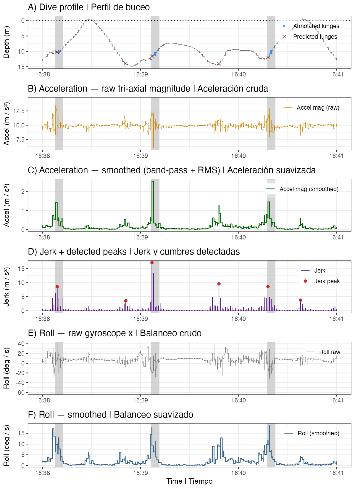
Note | Nota: the published figure also overlays manually annotated lunges (blue points) alongside the predicted ones, as a validation check against hand-scored data. | La figura publicada también superpone embestidas anotadas manualmente (puntos azules) junto a las predichas, como validación frente a datos revisados a mano.
References | Referencias
Cade, D. E., Friedlaender, A. S., Calambokidis, J., & Goldbogen, J. A. (2016). Kinematic diversity in rorqual whale feeding mechanisms. Current Biology, 26(19), 2617–2624.
Cade, D. E., Barr, K. R., Calambokidis, J., Friedlaender, A. S., & Goldbogen, J. A. (2018). Determining forward speed from accelerometer jiggle in aquatic environments. Journal of Experimental Biology, 221(2), jeb170449.
Goldbogen, J. A., Calambokidis, J., Shadwick, R. E., Oleson, E. M., McDonald, M. A., & Hildebrand, J. A. (2006). Kinematics of foraging dives and lunge-feeding in fin whales. Journal of Experimental Biology, 209(7), 1231–1244.
Goldbogen, J. A., Calambokidis, J., Friedlaender, A. S., Francis, J., DeRuiter, S. L., Stimpert, A. K., Falcone, E., & Southall, B. L. (2013). Underwater acrobatics by the world’s largest predator: 360° rolling manoeuvres by lunge-feeding blue whales. Biology Letters, 9(1), 20120986.
Owen, K., Dunlop, R. A., Monty, J. P., Chung, D., Noad, M. J., Donnelly, D., Goldizen, A. W., & Mackenzie, T. (2016). Detecting surface‐feeding behavior by rorqual whales in accelerometer data. Marine Mammal Science, 32(1), 327–348.x
Sweeney, D. A., DeRuiter, S. L., McNamara-Oh, Y. J., Marques, T. A., Arranz, P., & Calambokidis, J. (2019). Automated peak detection method for behavioral event identification: Detecting Balaenoptera musculus and Grampus griseus feeding attempts. Animal Biotelemetry, 7(1), 7.