Categorising residency and non-residency (movement) in acoustic telemetry data using basic dplyr functions
Author
Pablo Fuenzalida
Published
June 21, 2026
Hiya folks! My website may be written by AI, but this is not, so enjoy. To toggle dark / light mode, please hit the lil button on the top-right corner.
It’s me, your internet friend, Pablo :). If you’re reading this, thanks for exploring my first R tutorial!
I thought I’d kick it off with something easy(ish), yet useful - movement for acoustic telemetry.
I actually only learned about the data type in my third year of studying animal ecology, and was really interested in the many ways you could utilise the data, as well as the fact tags can last up to 10 years! It helps being an Aussie, we have IMOS - the Integrated Marine Observing System, which holds one of the largest repositories of animal movement in the world.
One of the many devious tasks associated with wrestling acoustic telemetry, is categorising movement. Relying on packages can simplify life, until they break….
So, I wrote some simple code in dplyr to define non-residency (movement between two detections), and residency (multiple detections at one receiver / array).
Let’s begin by downloading an IMOS toolkit REMORA (https://github.com/IMOS-AnimalTracking/remora), and loading some dummy data:
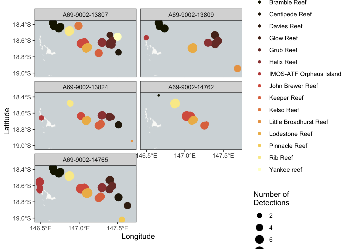
# requires a semi-newest version of R, and your ability to install this# for the sake of this tutorial being online, I'm blocking these out# however, if you do not have these packages install, run these lines# install.packages("remotes")# install.packages('pacman')# remotes::install_github('IMOS-AnimalTracking/remora',#build_vignettes = TRUE, # vignettes offline#dependencies = TRUE) # dependecies offlinelibrary('remora')library("tidyverse") # data wrestlinglibrary("terra") # spatial wrestlinglibrary("ggspatial") # mapslibrary('scico') # sexy colours library('plotly') #interative plots## Example dataset that has undergone quality control using the `runQC()` functiondata("TownsvilleReefQC")## Only retain detections flagged as 'valid' and 'likely valid' (Detection_QC 1 and 2)dat <- TownsvilleReefQC %>% tidyr::unnest(cols = QC) %>% dplyr::ungroup() %>%filter(Detection_QC %in%c(1,2))# dplyr wrestlingdat1 <- dat %>%group_by(transmitter_id, station_name, installation_name, receiver_deployment_longitude, receiver_deployment_latitude) %>%summarise(num_det =n()) %>% ungroup# ggplot it babyggplot(dat1) +annotation_map_tile('cartolight') +geom_spatial_point(aes(x = receiver_deployment_longitude, y = receiver_deployment_latitude, size = num_det, colour = installation_name), crs =4326) +facet_wrap(~transmitter_id, ncol =2) +labs(x ="Longitude", y ="Latitude", color ="Installation Name" , size ="Number of\nDetections") +theme_bw() +scale_colour_scico_d(palette ='lajolla')+scale_y_continuous(n.breaks =3)+scale_x_continuous(n.breaks =3)
# to look at the array in finer, interactive manners, we can rely on sf and mapviewdatxy <- dat %>%group_by(station_name, receiver_deployment_longitude, receiver_deployment_latitude) %>%summarise(num_det =n(), .groups ='drop')IMOSxy_sf <- sf::st_as_sf(datxy, coords =c("receiver_deployment_longitude", # need sf package"receiver_deployment_latitude"),crs =4326, agr ="constant")mapview::mapview(IMOSxy_sf, cex ="num_det", zcol ="station_name", fbg =FALSE) # need mapview package
Great, we have around 3 years of data across a few islands on the great barrier reef for 5 tags. Let’s get to making non-residency, aka movement.
Movement uses two detections, and denotes when it leaves one (departure), and arrives at another (arrival). From this information, we get: - date / time of both departure and arrival - location of both places - distance of the movement - time spent moving - Cardinal direction
Most of those are relevant for the common movement studies, some metrics more than others. To do this, we will use dplyr.
We shall group by our desired data (tag_id, time, locations etc.), and use dplyr’s lead / lag, to count between two subsequent rows in a tidy table, which finds the first detection, then connects it to the next. The rest, simple.
dat1 <- dat %>%transmute(tag_id = transmitter_id,datetime = detection_datetime, station_name = receiver_name,latitude = receiver_deployment_latitude,longitude = receiver_deployment_longitude,sex = animal_sex) %>%mutate(tag_id =as.character(tag_id)) %>%filter(if_all(everything(), ~!is.na(.))) # remove NAs and their entire rowanyNA(dat1) # needs to be false
# format should be: # tag id = character# datetime = POSIXct# location = character# station name = chr# lat / lon = numeric# sex = chr# non-residency -----------------------------------------------------------move_base <- dat1 %>%arrange(tag_id, datetime) %>%# arrange by ID and timegroup_by(tag_id) %>%# process data by tag ID, don't mix IDsmutate(next_time =lead(datetime), # lead time (lead / lag connects two rows (detections) that have already been arranged by time)next_station_name =lead(station_name), # lead location name, can be changed to receivernext_latitude =lead(latitude), # lat next_longitude =lead(longitude)) %>%# lon# Define a movement as a change in locationfilter(!is.na(next_station_name), station_name != next_station_name) %>%# filter movements that go to the same location (my methods but you can remove)mutate(movement_id =row_number()) %>%# movement_id to connect an arrival / departure movement as one in future ungroup() # lead created data for detecion 2, and replicated all variables# we now use this dataframe to create arrival and departure data# departures are detection 1, arrivals are detection 2 in a 'non-residency' or 'movement'# we then use bind_rows to connect them # the output gives us one row per arrival / departure, with all data we need# Departure rows creationdepartures <- move_base %>%transmute(tag_id, # transmute brings over data, arranges in order, and keeps str as well as renames all in onedatetime = datetime, # first datetime val in the dataframesex = sex,station_name = station_name,latitude = latitude,longitude = longitude,movement ="departure", movement_id)# Arrival rowsarrivals <- move_base %>%transmute(tag_id, # transmute brings over data, arranges in order, and keeps str as well as renames all in onedatetime = next_time,sex = sex,station_name = next_station_name,latitude = next_latitude,longitude = next_longitude,movement ="arrival", movement_id)# Combinedat2 <-bind_rows(departures, arrivals) %>%# departure and arrival dataframes should be the same size in obs (they're halfs of the same df movebase)arrange(tag_id, movement_id, movement, datetime)str(dat2)
# dat2 should be double the obs of movebase# since all we did was split rows of a movement into two: arrivals and depaturesdat2 %>%select(tag_id, station_name,movement,datetime) %>%arrange(tag_id, datetime, movement, station_name) %>%print(n =15)
Great! That worked, now let’s do residency. Residency has a lot of different meanings (https://link.springer.com/content/pdf/10.1186/s40462-022-00364-z.pdf), so make sure you read up on what you want to ask, and how you want to calculate that. I wanted to look at long-term residency, so I set minimum detections to be two a day, and a minimum of two days to categorise a residency ‘event’.
The way we do this, is very simple and again with dplyr. We will use the functions group_by and arrange to again format our data as we wish, then an if_else statement within mutate let’s us see if minimum numbers of our thresholds have been met, if they have, we make new columns for our ‘residency’! We also use functions like filter, summarise, and select to clean up our outputs and present them nicely.
min_detections_per_day <-2# minimum detections required on each daymin_res_days <-2# minimum length of residency in days (calendar, inclusive)max_gap_secs <-60*60*24# 1 day in seconds# residency ------------------------------------------------------------residency <- dat1 %>%arrange(tag_id, station_name, datetime) %>%group_by(tag_id, station_name) %>%mutate(time_gap =as.numeric(difftime(datetime, lag(datetime), units ="secs")),new_event =ifelse(is.na(time_gap) | time_gap > max_gap_secs, 1L, 0L),event_id =cumsum(replace_na(new_event, 1L))) %>%ungroup() %>%group_by(tag_id, station_name, event_id) %>%# compute daily stats within each eventmutate(day =as_date(datetime)) %>%summarise(start_datetime =min(datetime),end_datetime =max(datetime),start_day =min(day),end_day =max(day),n_days_incl =as.integer(end_day - start_day) +1L, # inclusive day spann_detections =n(),# per-day detection countsdays_meeting_threshold =sum( tapply(rep(1, n()), day, length) >= min_detections_per_day),sex =first(sex),.groups ="drop_last") %>%# keep events that last long enough AND meet the per-day threshold on every dayfilter(n_days_incl >= min_res_days, days_meeting_threshold == n_days_incl) %>%ungroup() %>%arrange(tag_id, start_datetime) %>%select(-c(n_days_incl))unique(residency$station_name)
Fantastic, we found two residency events longer than our minimum thresholds. This were two days each, one had four detections and one had five! You can tweak your input minimums based on what kinda ‘residency’ you want to define, and detect.
That’s all I have for you now, it’s late, and I want to sleep.