# 1 1 1 1 1
# 1 5 4 1 1
# 1 1 3 1 1
# 1 1 1 1 1 SST gradients as a proxy for dynamic ocean features
movement
spatial
oceanography
This tutorial calculates SST gradient using a centred finite differences approach (3x3) to estimate gradients in the form of °C km⁻¹ as a simple frontal proxy.
G’day friends. It’s been a few months since my last tutorial, and since I’m learning a new skill, I’d thought I would share this knowledge with you all at the same time.
Dynamic ocean features govern the high seas. When I was young I might’ve thought the deep ocean was one vast plain of the same environment, but since learning under scientists like Kylie Scales, I now know this to be quite false. The ocean is a dynamic seascape, temperature varies with depth, ocean currents swirl cool or warm water around the globe driven by predictable winds that we used to sail on.
As I move further into the world of animal movement, quantifying dynamic ocean features becomes increasingly important, especially in the context of marine megafauna movement. There is a plethora of literature showing environmental features can and do driver varies marine taxa to move across multiple contexts, and things like ocean eddys and fronts are one of those drivers. The rate of change might attract tiny fish to live in the warm or cold water, which brings bigger ones, and bigger ones eat those middle ones etc. etc. etc.
An eddy is a water body moving in a swirl, it’s direction depends on the coriolis effect so if you’re in the northern or southern hemisphere, they change. A front is slightly different, and we know them well in weather forecasts as warm or cold fronts passing through areas bringing about a steep change in temperature amongst other things. This is the same idea in-water, fronts bring about steep changes in temperature gradients, and vary in size. We have all these fancy words to quantify these things, and create various products depending on the context such as finite sized lyaponuv exponents (FSLE) to measure how particles stretch or contract in the ocean, which could be a proxy for both eddys and fronts.
Now before I go off on a long-ass story describing oceanography 101 as an ecologist, I’ve been taught to keep things as simple as possible without confounding the goal (to paraphrase Einstein). So, today, we shall demonstrate how to quantify a front signal in sea surface temperature data, using a simple gradient between cells calculation.
For me in my current context, I’m interested to see whether turtles are displaying more ‘foraging’ behaviour near these dynamic ocean features, so we need an environmental product that finds them!
Fronts change temperature very quickly in a small space, but they move, they are not static like an underwater mountain or an island.
Let’s say we have a 5 x 5 grid:
We can see that the values remain the same for most of the grid, except for the middle, there are some higher numbers. That means, spatially there is probably a numerical ‘front’ in those two rows with the values 5, 4, and 3. Now that might move the next day:
# 1 1 1 1 1
# 1 1 5 4 1
# 1 1 1 3 1
# 1 1 1 1 1
to the cells to the right, so we can see it shifts in space and time. It could shift in structure too:
# 1 1 1 1 1
# 1 1 5 4 3
# 1 1 1 1 1
# 1 1 1 1 1
It is now more straight compared to an angle. Now we can see these on a map, and we understand how dynamic they are, let’s find a way to delinate those areas where change is the steepest.
To find them, we must use some maths to calculate the difference between each cell within a given matrix, and see where values change quickly. For the purpose of this excercise, I’ve used generative AI to write me some code that mimics a dynamic but steep change in temperature within a grid
n <- 80L # 80 as an integer

library(terra)

sst <- terra::rast( # lets make a raster
  ncols = n, # n = 80 for columns
  nrows = n, # another 80 rows
  xmin = 170, # some bounding box values
  xmax = 170.5,
  ymin = -45,
  ymax = -44.5,
  crs = "EPSG:4326" # this is a spatial box so it needs a coordinate reference system
)

ex <- ext(sst) # let's make an extent

xy <- terra::xyFromCell(sst, 1:ncell(sst)) # lon/lat at the centre of every cell
lon <- xy[, 1] # longitudes (one number per cell)
lat <- xy[, 2] # latitudes (one number per cell)
lon_n <- (lon - ex[1]) / (ex[2] - ex[1]) # 0 = west edge, 1 = east edge
lat_n <- (lat - ex[3]) / (ex[4] - ex[3]) # 0 = south edge, 1 = north edge
edge_taper <- pmin( # fade the front off near the rim so margins stay ~19 °C
  pmin(lon_n / 0.15, (1 - lon_n) / 0.15), # west/east: full strength after 15% in from edge
  pmin(lat_n / 0.15, (1 - lat_n) / 0.15), # south/north: same
  1 # never above 1
)
front_lon <- 170.25 + 0.012 * sin((lat_n - 0.5) * 2 * pi * 3) # wavy front line (°E), moves with latitude
sst_vals <- 19 + 0.35 * tanh(-(lon - front_lon) / 0.008) * edge_taper # 19 °C ocean + small smooth step at front
terra::values(sst) <- sst_vals # write those temperatures into the raster
c(res_lon_deg = terra::res(sst)[1], # cell width in degrees (longitude)
  res_lat_deg = terra::res(sst)[2], # cell height in degrees (latitude)
  sst_min = min(sst_vals), # coolest cell (sanity check)
  sst_max = max(sst_vals)) # warmest cell (sanity check)
res_lon_deg res_lat_deg sst_min sst_max
0.00625 0.00625 18.65000 19.35000 plot(sst, main = "A dynamic SST ocean")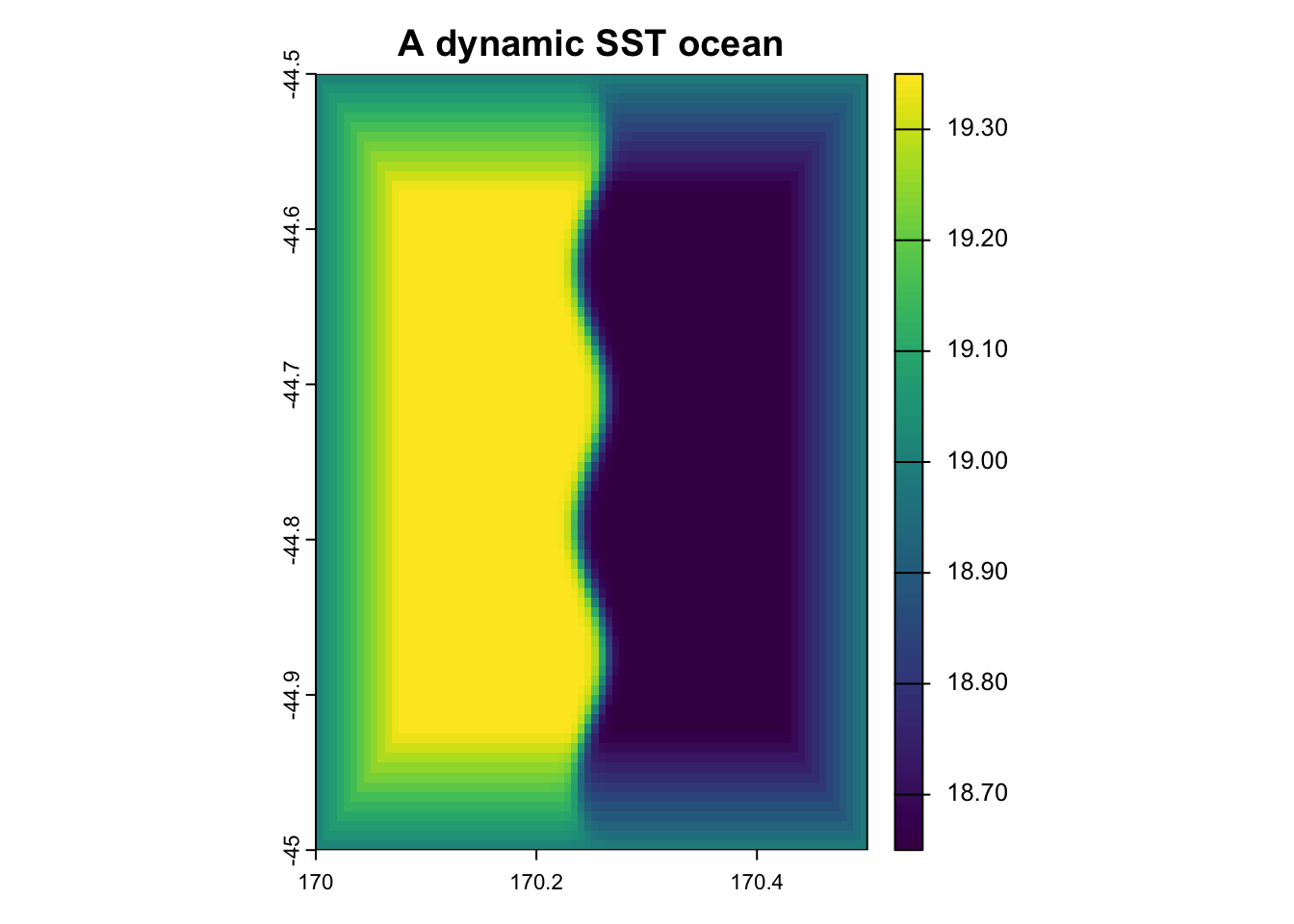
Now apart from that being very aesthetically pleasing with a (new) base colour of viridis, we have a good example of how a front may present itself in some data.
Now what we want from this, is to find in this grid cell the place where values change the quickest. We can call this the steepest gradient, or magnitude gradient.
Now we have the basics, let’s begin wrestling.
First step is to change our cell size from degrees, into kilometres so we can create a product that shows the rate of change in celcius per km-1 instead of celcius per cell (which isn’t very informative).
res <- terra::res(sst) # resolution of the cell eg. width in ° lon, height in ° lat

clat <- mean( # one average latitude for the whole patch (degrees north)
  terra::yFromCell(sst, seq_len(min(5000L, terra::ncell(sst)))), # lat at each cell centre (cap at 5000cells)
  na.rm = TRUE) # ignore NA latitudes if any

# 111.32 is the average length of a degree across the planet in km
# obvs this stretches and contracts depending on your latitudional positioning on the planet
# because it is round (sorry to say)

dx_km <- as.numeric(res[1]) * 111.32 * cos(clat * pi / 180) # east–west km per cell (shrinks toward poles)
dy_km <- as.numeric(res[2]) * 111.32 # north–south km per cell (~111 km per degree lat)

c(dx_km = dx_km, dy_km = dy_km, mean_lat = clat) # print so you can check before |∇SST|
dx_km dy_km mean_lat
0.4945787 0.6957500 -44.6953250 # so the values below, are on average 0.49km wide for x and 0.69 km wide for yGreat! We have now transformed this cell from degrees to kilometers, using the latitude and longitude of the bounding box set earlier.
This will change for your study site depending on where you are in the planet, so if your values are different to these, good. They should be.
The next step, now that we have our ducks in a row, is to calculate the gradient between cells. We will do this using a 3 x 3 cell mesh filter, bascially saying grab a 3 x 3 grid and use the variation within that area to delinate where values are changing the most quickly.
sst_gradient_finder <- function(sst) { #we need a name for our function
  if (is.null(sst) || !terra::ncell(sst)) return(NULL) # if sst is empty, return empty values

  res <- terra::res(sst) # get sst resolution
  clat <- mean( # grab the mean into the centre latitude
    terra::yFromCell(sst, seq_len(min(5000L, terra::ncell(sst)))), #grab y coordinates from a cell
    # and build a list of cell IDs and ask for the lat of each of those
    na.rm = TRUE) # remove NAs from this space

  dx_km <- as.numeric(res[1]) * 111.32 * cos(clat * pi / 180) # calc a  val of km per cell from east-west
  dy_km <- as.numeric(res[2]) * 111.32 # no cos-sign transformation needed for a north-south km cell calc
  if (!is.finite(dx_km) || dx_km <= 0 || !is.finite(dy_km) || dy_km <= 0) return(NULL)
  # FYI, when using two || it means OR in R-language (baseR)
  # so we're saying if dx_km is NaN or infinite (broken)
  # or if kx_km is the same or less than 0 in east-west or north-south
  # return a null, so we know its broken

  # now we make our matrix of 3 x 3
  w_x <- matrix(c(0, 0, 0, -0.5, 0, 0.5, 0, 0, 0), nrow = 3, ncol = 3) # centred ∂/∂x stencil (middle row)
  w_y <- matrix(c(0, -0.5, 0, 0, 0, 0, 0, 0.5, 0), nrow = 3, ncol = 3) # centred ∂/∂y stencil (middle column)
  # where  ∂ is a partial derivative
  # which is a fancy term for saying how we calculate
  # the change in temperature per step in space, not time
  # so the first line w_x calculates the rate of change across longitude (columns in data)
  # the second w_y, across latitude (rows in data)
  # you can write this in a formula as: grad_SST = √((∂SST/∂x)² + (∂SST/∂y)²)
  # for those freaky aah mathematician

  # this next part is conceptually fun, we're creating a window 'slider' which moves over cells
  # and weighs each side by 0.5 (plus and minus)
  # then we find the difference by using those weights to see how values change in the 3 x 3
  # focal does this, based inside terra (lovely spatial package, goodbye ol' Raster)

  gx <- terra::focal(sst, # find the focal point of sst
                     w = w_x, # our width is longitude
                     fun = sum, # the function is the sum of values inside the cell
                     na.rm = TRUE, # remove NAs
                     pad = TRUE) / dx_km # °C/km in x, and pad raster edges

  # this is the same, for y, I won't write each bit out
  gy <- terra::focal(sst, w = w_y, fun = sum, na.rm = TRUE, pad = TRUE) / dy_km

  # now we must square-root the output to combine both X and Y slopes
  # they currently live as magnitudes, pythagoras says we can bring them together by square-root

  sqrt(gx^2 +  # square-root x to the power of 2
         gy^2) # and y to the power of 2

  } # finish the function

grad <- sst_gradient_finder(sst) # run it on our toy ocean
plot(grad)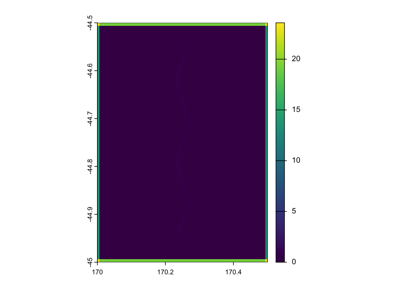
# there is a very faint line in the middle, but the edges mask it
# lets crop the edges to see that faint line
# in your study, the edges shouldn't be changing like these ones do
# its only because this is fake data
# Mask outer rim for plotting only (focal pad can inflate |∇SST| on the frame).
gradient_complete <- grad
edge <- lon_n < 0.08 | lon_n > 0.92 | lat_n < 0.08 | lat_n > 0.92 # trim edges
gvals <- terra::values(gradient_complete) # bring vals into gvals
gvals[edge] <- NA # fill edges with NA
terra::values(gradient_complete) <- gvals # return back into a values terra obj

plot(gradient_complete) # plot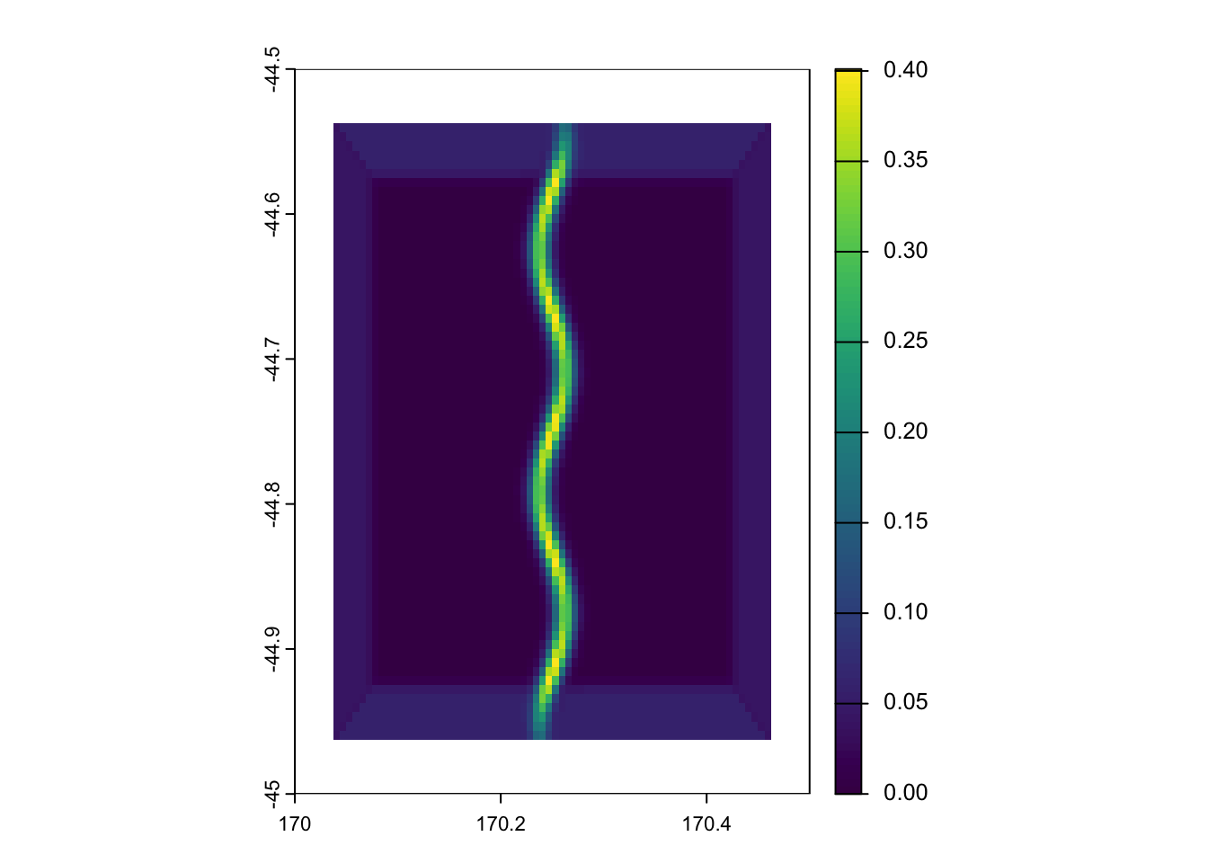
Nice job! We have sucessfully found the values in this cell that have a steep change in their values in a small area, the gradient!
It looks different as we cropped the edges to illuminate the gradient in the middle.
To plot this together with our first map, we can use the baseR function par
par(mfrow = c(1, 2)) # two objects plotted together
plot(sst)
plot(gradient_complete)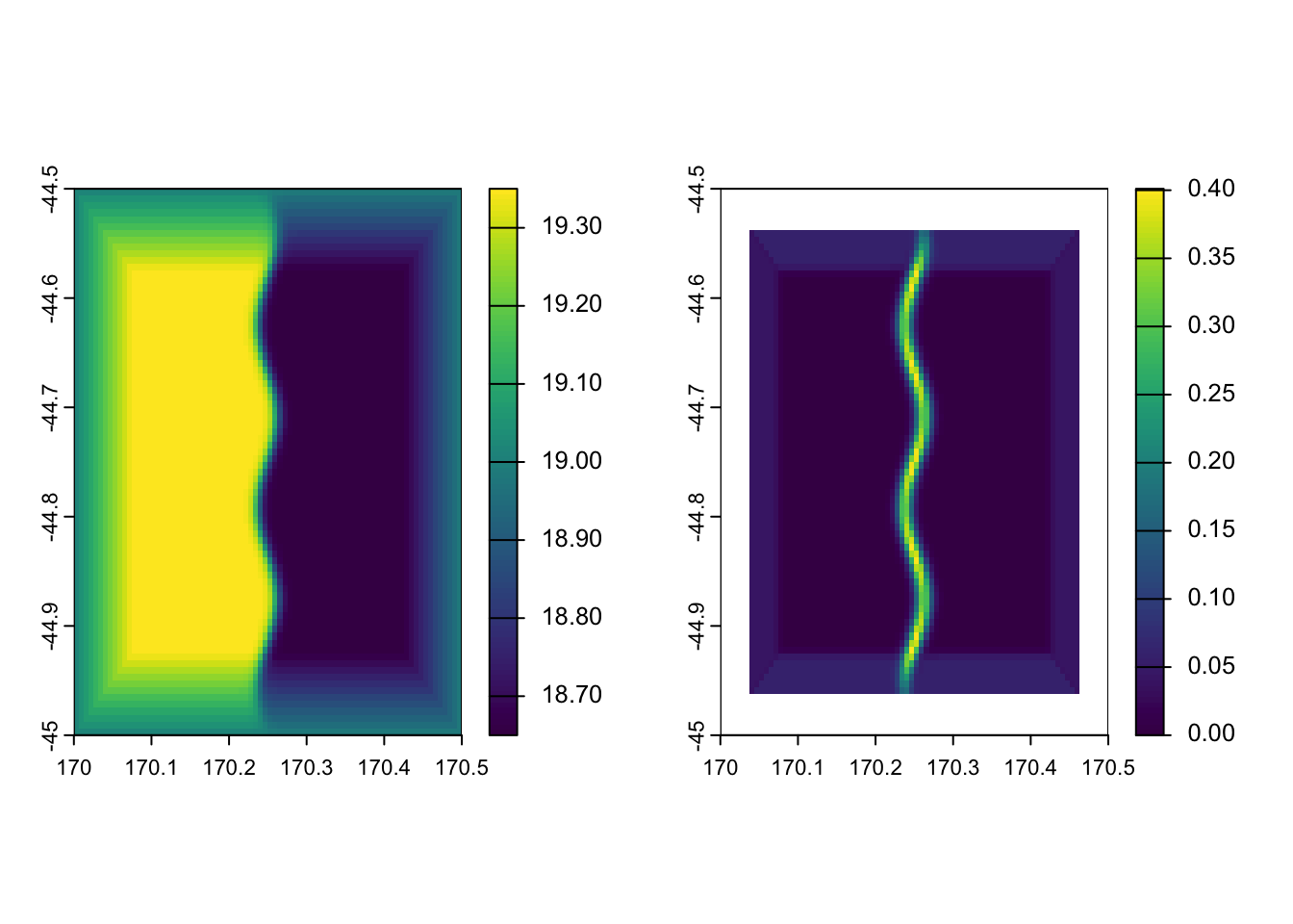
# run this togetherTada! How friggen cool dude, stoked!
You can see on the left pane, maybe two oceans meeting or two bodies of water at starkly different temperatures (above 19 °C and below 18.8 °C in this instance), and on the right, you can see the thermal gradient (in °C km⁻¹ as we so intelligently transformed it).
This is a very simple step by step way one doing this, you can calculate these gradients using netcdfs of SST if you already downloaded those layers and cached them locally, without having to hop back onto data holders portals / websites / packages and re-download something else…
I do want to caution before wrapping up, this is the simpliest form of calculating a SST gradient I can currently think of. This may not pick up fine-scale ocean features, this is a proxy for fronts, not a ‘front detector’. This probably picks up mesoscale fronts on a km scale of 50 - 100km +, but smaller things won’t be found with this approach. It also depends on your SST product, and whether it was smoothed beforehand, but that’s an oceanographers problem, which means talking to them (and you should try to avoid that as an ecologist). If this is computed on a daily scale, you also need to think about the temporal aspect, are you doing to smoothen this across days, weeks, months? How will a moving front affect this process? Our magnitude does not compute direction, but if values in the grid are there, which way is it moving? Is it co-linear with other variables in our statistical model? How much padding is too much in these gradients?
I have dabbled in various appraoches to this previously, but due to time constraints (and limited tracks), will be using this simple analysis as a bit of an exploratory proxy for fronts in my own paper which I hope to publish in the near future.
I want to thank Josh E. Esman (AKA big dawg) for his guidance on how he approaches calculating frontal proxies. Perhaps in the near-future he will be the first ‘guest’ in our R blog writing a more complicated approach to this.
For now, stay chill my friends. Life is one terrifying joyous ride, don’t add to the suffering.
Best fishes,
Pablo